Search vs. planning Consider the task get milk, bananas, and a - - PowerPoint PPT Presentation

Planning

Chapter 11

Chapter 11 1

Outline

♦ Search vs. planning ♦ STRIPS operators ♦ Partial-order planning

Chapter 11 2

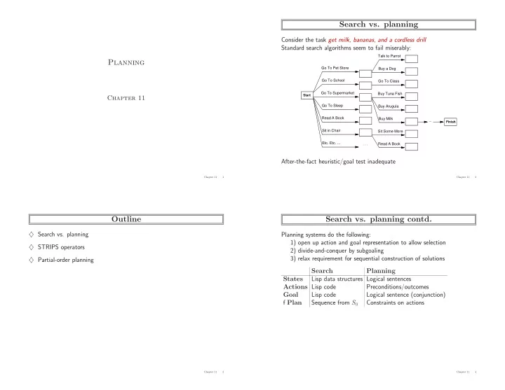
Search vs. planning

Consider the task get milk, bananas, and a cordless drill Standard search algorithms seem to fail miserably:

. . .

Buy Tuna Fish Buy Arugula Buy Milk Go To Class Buy a Dog Talk to Parrot Sit Some More Read A Book

...

Go To Supermarket Go To Sleep Read A Book Go To School Go To Pet Store

• Etc. Etc. ...

Sit in Chair

Start Finish

After-the-fact heuristic/goal test inadequate

Chapter 11 3

Search vs. planning contd.

Planning systems do the following: 1) open up action and goal representation to allow selection 2) divide-and-conquer by subgoaling 3) relax requirement for sequential construction of solutions Search Planning States Lisp data structures Logical sentences Actions Lisp code Preconditions/outcomes Goal Lisp code Logical sentence (conjunction) f Plan Sequence from S0 Constraints on actions

Chapter 11 4

STRIPS operators

Tidily arranged actions descriptions, restricted language Action: Buy(x)

Have(x) At(p) Sells(p,x)

Buy(x)

Precondition: At(p), Sells(p, x) Effect: Have(x) [Note: this abstracts away many important details!] Restricted language ⇒ efficient algorithm

• Precondition: conjunction of positive literals
• Effect: conjunction of literals

– postive effect: add literals – negative effect: remove literals (negated literals)

Chapter 11 5

Forward State-space Search

♦ aka Progression Planning ♦ similar to Forward Chaining ♦ State-space formulation

• Initial State: initial KB
• Actions: operators whose preconditions are satisfied

– successors: ∗ postive effect: add literals ∗ negative effect: remove literals

• Goal test: goal state
• Step cost: typically 1

Chapter 11 6

Backward State-space Search

♦ aka Regression Planning ♦ similar to Backward Chaining ♦ Difficult if the goal is described as constraints (e.g. 4 gallons in the large jug)—potentially many goal states. ♦ A goal can be divided into sub-goals (children). ♦ State-space formulation

• Initial State: goal state
• Actions: operations that can acheive the goal/sub-goal

– not undo any super-goals [parent goals/preconditions] – succesors: ∗ sub-goals (unsatisfied precoditions)

• Goal test: no sub-goals (no unsatisfied preconditions)

Chapter 11 7

Admissible Heuristics

♦ Relaxed problem

• remove all precoditions—every action is applicable
• remove all negative effects—no action removes a literal

(note that the goal is a conjuction of literals)

• subgoal independence—achieving one subgoal does not affect achieving

another subgoal

Chapter 11 8

Partial Order Planning

♦ sequential planning: forward (or backward) step-by-step search ♦ Consider planning a trip to New York by flying

• 1. start with finding how to get from home to the Melboune airport
• 2. start with finding how to get from the New York airport to hotel
• 3. start with finding a plane ticket from Melbourne to New York

♦ least commitment strategy—delay making committments to steps that are less important/constrained

Chapter 11 9

Partial Order Planning

LeftSockOn RightSockOn LeftShoeOn, RightShoeOn Start Sock Right Shoe Right Sock Left Shoe Left Finish

Finish Start

LeftShoeOn, RightShoeOn

Chapter 11 10

Components of Partial Order Planning

• Actions

– “Start” action: no preconditions, effects = initial state – “Finish” action: preconditions = goal state, no effects – (regular) actions with precondtions and effects

• Ordering contraints between actions

– A ≺ B: A is before B (partial order) – LeftSock ≺ LeftShoe

• Causal links from effect of one action to the precondition of another

– A

c

− → B: A acheives precondition c for B – LeftSock LeftSockOn − → LeftShoe – other actions cannot conflict with the causal link: ¬LeftSockOn

• Open preconditions

– not acheived by any action yet – planner: add actions until there are no open preconditions

Chapter 11 11

Example

Finish Start At(Home) Have(Ban.) Have(Drill) Have(Milk) Sells(SM,Milk) Sells(HWS,Drill) At(Home) Sells(SM,Ban.)

Chapter 11 12

Example

Buy(Drill) Buy(Milk) Go(SM) Finish Start At(Home) Have(Ban.) Have(Drill) Have(Milk) Sells(SM,Milk) At(SM) Sells(HWS,Drill) At(HWS) At(x) Sells(SM,Milk) Sells(HWS,Drill) At(Home) Sells(SM,Ban.)

Chapter 11 13

Example

At(SM) At(Home) At(HWS) Buy(Drill) Buy(Milk) Buy(Ban.) Go(Home) Go(HWS) Go(SM) Finish Start At(Home) Have(Ban.) Have(Drill) Have(Milk) Sells(SM,Milk) At(SM) Sells(SM,Ban.) At(SM) Sells(HWS,Drill) At(HWS)

Chapter 11 14

Planning process

Operators on partial plans: add a link from an existing action to an open condition add a step to fulfill an open condition

• rder one step wrt another to remove possible conflicts

Gradually move from incomplete/vague plans to complete, correct plans Backtrack if an open condition is unachievable or if a conflict is unresolvable Topological Sorting in graphs

Chapter 11 15

POP algorithm sketch

function POP(initial, goal, operators) returns plan plan ← Make-Minimal-Plan(initial, goal) loop do if Solution?( plan) then return plan Sneed, c ← Select-Subgoal( plan) Choose-Operator( plan, operators,Sneed,c) Resolve-Threats( plan) end function Select-Subgoal( plan) returns Sneed, c pick a plan step Sneed from Steps( plan) with a precondition c that has not been achieved return Sneed, c

Chapter 11 16

POP algorithm contd.

procedure Choose-Operator(plan, operators,Sneed, c) choose a step Sadd from operators or Steps( plan) that has c as an effect if there is no such step then fail add the causal link Sadd

c

− → Sneed to Links( plan) add the ordering constraint Sadd ≺ Sneed to Orderings( plan) if Sadd is a newly added step from operators then add Sadd to Steps( plan) add Start ≺ Sadd ≺ Finish to Orderings( plan) procedure Resolve-Threats(plan) for each Sthreat that threatens a link Si

c

− → Sj in Links( plan) do choose either Demotion: Add Sthreat ≺ Si to Orderings( plan) Promotion: Add Sj ≺ Sthreat to Orderings( plan) if not Consistent( plan) then fail end

Chapter 11 17

Clobbering and promotion/demotion

A clobberer is a potentially intervening step that destroys the condition achieved by a causal link. E.g., Go(Home) clobbers At(Supermarket):

Finish At(Home) At(Home) Go(Home) DEMOTION PROMOTION Go(Supermarket) At(Supermarket) Buy(Milk)

Demotion: put before Go(Supermarket) Promotion: put after Buy(Milk)

Chapter 11 18

Properties of POP

Nondeterministic algorithm: backtracks at choice points on failure: – choice of Sadd to achieve Sneed – choice of demotion or promotion for clobberer – selection of Sneed is irrevocable POP is sound, complete, and systematic (no repetition) Extensions for disjunction, universals, negation, conditionals Can be made efficient with good heuristics derived from problem description Particularly good for problems with many loosely related subgoals

Chapter 11 19

Example: Blocks world

Start State Goal State

B A C A B C

PutOn(x,y) Clear(x) On(x,z) Clear(y) ~On(x,z) ~Clear(y) Clear(z) On(x,y) PutOnTable(x) Clear(x) On(x,z) ~On(x,z) Clear(z) On(x,Table) + several inequality constraints

"Sussman anomaly" problem

[Linear planners (find a plan for each subgoal and concatenate the plans) can’t find a solution]

Chapter 11 20

Example contd.

B A C A B C

FINISH On(A,B) On(B,C) START On(C,A) On(A,Table) Cl(B) On(B,Table) Cl(C)

Chapter 11 21

Example contd.

B A C A B C

FINISH START On(C,A) On(A,Table) Cl(B) On(B,Table) Cl(C) PutOn(B,C) Cl(B) On(B,z) Cl(C) On(A,B) On(B,C)

Chapter 11 22

Example contd.

B A C A B C

FINISH On(A,B) On(B,C) START On(C,A) On(A,Table) Cl(B) On(B,Table) Cl(C) PutOn(B,C) PutOn(A,B)

PutOn(A,B) clobbers Cl(B) => order after PutOn(B,C)

On(A,z) Cl(B) Cl(A) On(B,z) Cl(C) Cl(B)

Chapter 11 23

Example contd.

B A C A B C

FINISH On(A,B) On(B,C) START On(C,A) On(A,Table) Cl(B) On(B,Table) Cl(C) PutOn(B,C) Cl(B) On(B,z) Cl(C) PutOn(A,B) Cl(A) On(A,z) Cl(B)

PutOn(A,B) clobbers Cl(B) => order after PutOn(B,C)

PutOnTable(C)

PutOn(B,C) clobbers Cl(C) => order after PutOnTable(C)

Cl(C) On(C,z)

Chapter 11 24

Heuristics

♦ Which open precondition to choose?

• most constrained open precondition

– can be satisfied in the fewest number of ways

• can provide substantial speedups

– if it can’t be satisfied, stop early and return fail – if it can be satisfied by only one way, no choice anyhow and can reduce the number of possibilities later on

Chapter 11 25