[PDF] - Search: Uninformed Search Russel & Norvig Chap. 3 Material in PDF Document

SLIDE 1

1

Search: Uninformed Search

Material in part from http://www.cs.cmu.edu/~awm/tutorials Russel & Norvig Chap. 3

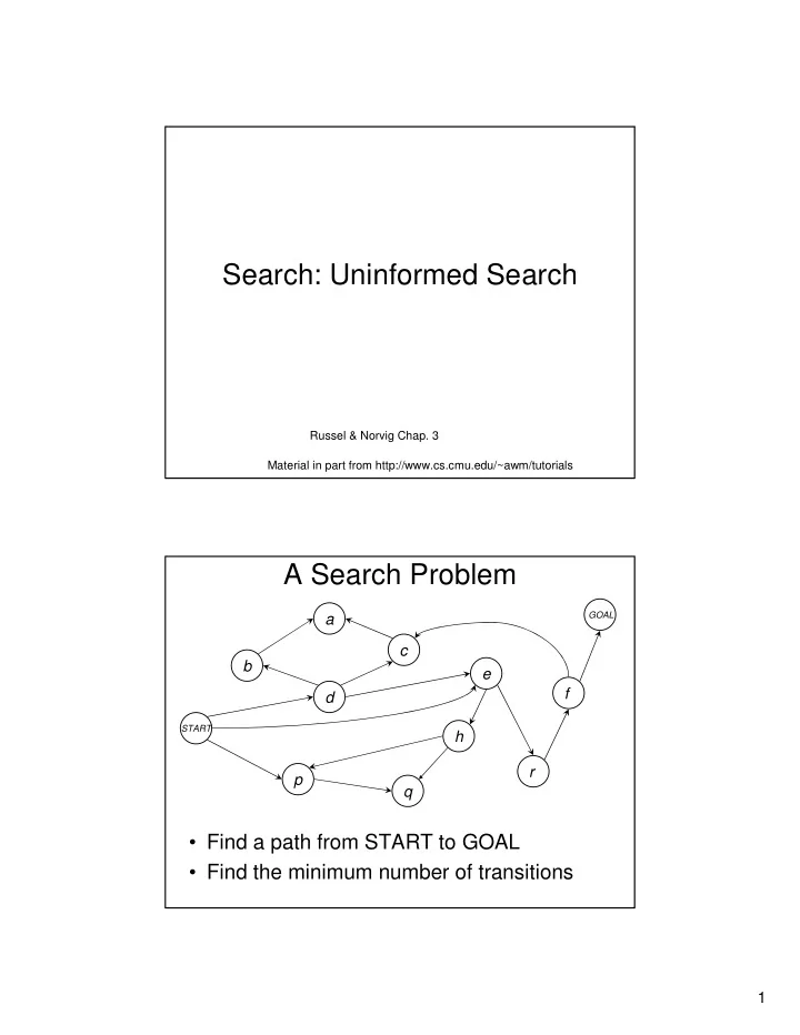
A Search Problem

Find a path from START to GOAL
Find the minimum number of transitions

b a d p q h e c f r

START GOAL

SLIDE 2

2

Example

2 8 3 1 6 4 7 5 2 8 3 1 6 4 7 5

START GOAL

Example

State: Configuration of puzzle
Transitions: Up to 4 possible moves (up, down,

left, right)

Solvable in 22 steps (average)
But: 1.8 105 states (1.3 1012 states for the 15-

puzzle) Cannot represent set of states explicitly

2 8 3 1 6 4 7 5 2 8 3 1 6 4 7 5

START GOAL

SLIDE 3

3

Example: Robot Navigation

X x

START GOAL

States = positions in the map Transitions = allowed motions

N E S W

Navigation: Going from point START to point GOAL given a (deterministic) map

Other Real-Life Examples

Protein design

http://www.blueprint.org/proteinfolding/trades/trades_problem.html

Scheduling/Manufacturing

http://www.ozone.ri.cmu.edu/projects/dms/dmsmain.html

Scheduling/Science

http://www.ozone.ri.cmu.edu/projects/hsts/hstsmain.html

Route planning Robot navigation

http://www.frc.ri.cmu.edu/projects/mars/dstar.html

Don’t necessarily know explicitly the structure of a search problem

SLIDE 4

4 10cm resolution 4km2 = 4 108 states

What we are not addressing (yet)

Uncertainty/Chance State and transitions are known and deterministic
Game against adversary
Multiple agents/Cooperation
Continuous state space For now, the set of states is discrete

SLIDE 5

5

Overview

Definition and formulation
Optimality, Completeness, and Complexity
Uninformed Search

– Breadth First Search – Search Trees – Depth First Search – Iterative Deepening

Informed Search

– Best First Greedy Search – Heuristic Search, A*

A Search Problem

b a d p q h e c f r

START GOAL

SLIDE 6

6

Formulation

Q: Finite set of states
S

Q: Non-empty set of start states

G

Q: Non-empty set of goal states

succs: function Q (Q)

succs(s) = Set of states that can be reached from s in one step

cost: function QxQ Positive Numbers

cost(s,s’) = Cost of taking a one-step transition from state s to state s’

Problem: Find a sequence {s1,…,sK} such that:
1. s1

S

2. sK

G

3. si+1

succs(si)

4. Σ cost(si, si+1) is the smallest among all possible

sequences (desirable but optional)

⊆ ⊆

∈ ∈ ∈

Example

Q = {START, GOAL, a, b, c, d, e, f, h, p, q, r}
S = {START} G = {GOAL}
succs(d) = {b,c}
succs(START) = {p,e,d}
succs(a) = NULL
cost(s,s’) = 1 for all transitions

b a d p q h e c f r

START GOAL

SLIDE 7

7

Desirable Properties

Completeness: An algorithm is complete if it is

guaranteed to find a path if one exists

Optimality: The total cost of the path is the lowest

among all possible paths from start to goal

Time Complexity
Space Complexity

b a d p q h e c f r

START GOAL

b a d p q h e c f r

START GOAL

Breadth-First Search

Label all states that are 0 steps from S

Call that set Vo

b a d p q h e c f r

START GOAL

SLIDE 8

8

Breadth-First Search

Label the successors of the states in Vo

that are not yet labelled Set V1 of states that are 1 step away from the start

b a d p q h e c f r

START GOAL

0 steps 1 step

Breadth-First Search

Label the successors of the states in V1

that are not yet labelled Set V2 of states that are 1 step away from the start

b a d p q h e c f r

START GOAL

0 steps 1 step 2 steps

SLIDE 9

9

Breadth-First Search

Label the successors of the states in V2

that are not yet labelled Set V3 of states that are 1 step away from the start

b a d p q h e c f r

START GOAL

0 steps 1 step 2 steps 3 steps

Breadth-First Search

Stop when goal is reached in the current

expansion set goal can be reached in 4 steps

b a d p q h e c f r

START GOAL

0 steps 1 step 2 steps 3 steps 4 steps

SLIDE 10

10

Recovering the Path

Record the predecessor state when labeling a new state
When I labeled GOAL, I was expanding the neighbors of

f f is the predecessor of GOAL

When I labeled f, I was expanding the neighbors of r r

is the predecessor of f

Final solution: {START, e, r, f, GOAL}

b a d p q h e c f r

START GOAL

Using Backpointers

A backpointer previous(s) point to the node that

stored the state that was expanded to label s

The path is recovered by following the

backpointers starting at the goal state

b a d p q h e c f r

START GOAL

SLIDE 11

11

Example: Robot Navigation

X x

START GOAL

States = positions in the map Transitions = allowed motions

N E S W

Navigation: Going from point START to point GOAL given a (deterministic) map

Breadth First Search

V0  S (the set of start states) previous(START) := NULL k  0 while (no goal state is in Vk and Vk is not empty) do

Vk+1  empty set For each state s in Vk

For each state s’ in succs(s)

If s’ has not already been labeled Set previous(s’)  s Add s’ into Vk+1

k  k+1

if Vk is empty signal FAILURE else build the solution path thus:

Define Sk = GOAL, and forall i <= k, define Si-1 = previous(Si) Return path = {S1,.., Sk}

SLIDE 12

12

Properties

BFS can handle multiple start and goal

states

Can work either by searching forward from

the start or backward for the goal (forward/backward chaining)

(Which way is better?)
Guaranteed to find the lowest-cost path in

terms of number of transitions??

See maze example

Complexity

N = Total number of states
B = Average number of successors (branching factor)
L = Length from start to goal with smallest number of steps

Breadth First Search BFS Space Time Optimal Complete Algorithm

SLIDE 13

13

V3 V’3

Bidirectional Search

BFS search simultaneously forward from

START and backward from GOAL

When do the two search meet?
What stopping criterion should be used?
Under what condition is it optimal?

START GOAL

V1 V’1 V2 V’2

Complexity

N = Total number of states
B = Average number of successors (branching factor)
L = Length for start to goal with smallest number of steps

Bi-directional Breadth First Search

BIBFS

Breadth First Search

BFS Space Time Optimal Complete Algorithm

B = 10, L = 6 22,200 states generated vs. ~107 Major savings when bidirectional search is possible because 2BL/2 << BL

SLIDE 14

14

Counting Transition Costs Instead of Transitions

b a d p q h e c f r

START GOAL

2 1 3 1 9 15 8 2 2 4 9 5 5 5 4 1 3

Counting Transition Costs Instead of Transitions

BFS finds the shortest path in number of steps but

does not take into account transition costs

Simple modification finds the least cost path
New field: At iteration k, g(s) = least cost path to s in k
r fewer steps

b a d p q h e c f r

START GOAL

2 1 3 1 9 15 8 2 2 4 9 5 5 5 4 1 3

SLIDE 15

15

Uniform Cost Search

Strategy to select state to expand next
Use the state with the smallest value of g()

so far

Use priority queue for efficient access to

minimum g at every iteration

Priority Queue

Priority queue = data structure in which data of

the form (item, value) can be inserted and the item of minimum value can be retrieved efficiently

Operations:

– Init (PQ): Initialize empty queue – Insert (PQ, item, value): Insert a pair in the queue – Pop (PQ): Returns the pair with the minimum value

In our case:

– item = state value = current cost g()

Complexity: O(log(number of pairs in PQ)) for insertion and pop operations very efficient

http://www.leekillough.com/heaps/ Knuth&Sedwick ….

SLIDE 16

16

Uniform Cost Search

PQ = Current set of evaluated states
Value (priority) of state = g(s) = current cost
f path to s
Basic iteration:
1. Pop the state s with the lowest path cost from PQ
2. Evaluate the path cost to all the successors of s
3. Add the successors of s to PQ

We add the successors of s that have not yet been visited and we update the cost of those currently in the queue b a d p q h e c f r

START GOAL

2 1 3 1 9 15 8 2 2 4 9 5 5 5 4 1 3

1. Pop the state s with the lowest path cost from PQ 2. Evaluate the path cost to all the successors of s 3. Add the successors of s to PQ

PQ = {(START,0)}

SLIDE 17

17 b a d p q h e c f r

START GOAL

2 1 3 1 9 15 8 2 2 4 9 5 5 5 4 1 3

1. Pop the state s with the lowest path cost from PQ 2. Evaluate the path cost to all the successors of s 3. Add the successors of s to PQ

PQ = {(p,1) (d,3) (e,9)}

b a d p q h e c f r

START GOAL

2 1 3 1 9 15 8 2 2 4 9 5 5 5 4 1 3

1. Pop the state s with the lowest path cost from PQ 2. Evaluate the path cost to all the successors of s 3. Add the successors of s to PQ

PQ = {(d,3) (e,9) (q,16)}

SLIDE 18

18 b a d p q h e c f r

START GOAL

2 1 3 1 9 15 8 2 2 4 9 5 5 5 4 1 3

1. Pop the state s with the lowest path cost from PQ 2. Evaluate the path cost to all the successors of s 3. Add the successors of s to PQ

PQ = {(b,4) (e,5) (c,11) (q,16)}

b a d p q h e c f r

START GOAL

2 1 3 1 9 15 8 2 2 4 9 5 5 5 4 1 3

1. Pop the state s with the lowest path cost from PQ 2. Evaluate the path cost to all the successors of s 3. Add the successors of s to PQ

PQ = {(b,4) (e,5) (c,11) (q,16)}

Important: We realized that going to e through d is cheaper than going to e directly the value of e is updated from 9 to 5 and it moves up in PQ

SLIDE 19

19 b a d p q h e c f r

START GOAL

2 1 3 1 9 15 8 2 2 4 9 5 5 5 4 1 3

1. Pop the state s with the lowest path cost from PQ 2. Evaluate the path cost to all the successors of s 3. Add the successors of s to PQ

PQ = {(e,5) (a,6) (c,11) (q,16)}

b a d p q h e c f r

START GOAL

2 1 3 1 9 15 8 2 2 4 9 5 5 5 4 1 3

1. Pop the state s with the lowest path cost from PQ 2. Evaluate the path cost to all the successors of s 3. Add the successors of s to PQ

PQ = {(a,6) (h,6) (c,11) (r,14) (q,16)}

SLIDE 20

20 b a d p q h e c f r

START GOAL

2 1 3 1 9 15 8 2 2 4 9 5 5 5 4 1 3

1. Pop the state s with the lowest path cost from PQ 2. Evaluate the path cost to all the successors of s 3. Add the successors of s t PQ

PQ = {(h,6) (c,11) (r,14) (q,16)}

b a d p q h e c f r

START GOAL

2 1 3 1 9 15 8 2 2 4 9 5 5 5 4 1 3

1. Pop the state s with the lowest path cost from PQ 2. Evaluate the path cost to all the successors of s 3. Add the successors of s to PQ

PQ = {(q,10) (c,11) (r,14)}

SLIDE 21

21 b a d p q h e c f r

START GOAL

2 1 3 1 9 15 8 2 2 4 9 5 5 5 4 1 3

1. Pop the state s with the lowest path cost from PQ 2. Evaluate the path cost to all the successors of s 3. Add the successors of s to PQ

PQ = {(q,10) (c,11) (r,14)}

Important: We realized that going to q through h is cheaper than going through p the value of q is updated from 16 to 10 and it moves up in PQ b a d p q h e c f r

START GOAL

2 1 3 1 9 15 8 2 2 4 9 5 5 5 4 1 3

PQ = {(c,11) (r,13)}

1. Pop the state s with the lowest path cost from PQ 2. Evaluate the path cost to all the successors of s 3. Add the successors of s to PQ

SLIDE 22

22 b a d p q h e c f r

START GOAL

2 1 3 1 9 15 8 2 2 4 9 5 5 5 4 1 3

PQ = {(r,13)}

1. Pop the state s with the lowest path cost from PQ 2. Evaluate the path cost to all the successors of s 3. Add the successors of s to PQ

PQ = {(f,18)}

b a d p q h e c f r

START GOAL

2 1 3 1 9 15 8 2 2 4 9 5 5 5 4 1 3

1. Pop the state s with the lowest path cost from PQ 2. Evaluate the path cost to all the successors of s 3. Add the successors of s to PQ

PQ = {(GOAL,23)}

SLIDE 23

23 b a d p q h e c f r

START GOAL

2 1 3 1 9 15 8 2 2 4 9 5 5 5 4 1 3 Final path: {START, d, e, h, q, r, f, GOAL}

This path is optimal in total cost even though it has more

transitions than the one found by BFS

What should be the stopping condition?
Under what conditions is UCS complete/optimal?

Example: Robot Navigation

X x

START GOAL

States = positions in the map Transitions = allowed motions

N E S W

Navigation: Going from point START to point GOAL given a (deterministic) map Cost = sqrt(2) Cost = 1

SLIDE 24

24

Complexity

N = Total number of states
B = Average number of successors (branching factor)
L = Length for start to goal with smallest number of steps
Q = Average size of the priority queue

Bi-directional Breadth First Search BIBFS Uniform Cost Search UCS Breadth First Search BFS

Space Time Optimal Complete Algorithm

Limitations of BFS

Memory usage is O(BL) in general
Limitation in many problems in which the

states cannot be enumerated or stored explicitly, e.g., large branching factor

Alternative: Find a search strategy that

requires little storage for use in large problems

SLIDE 25

25

Depth First Search

General idea:

– Expand the most recently expanded node if it has successors – Otherwise backup to the previous node on the current path

START START d START d b START d b a START d c START d c a START d e START d e r START d e r f START d e r f c START d e r f c a START d e r f GOAL

b a d p q h e c f r

GOAL START

DFS Implementation

DFS (s)

if s = GOAL

return SUCCESS

else

For all s’ in succs(s)

DFS (s’)

return FAILURE

In a recursive implementation, the program stack keeps track of the states in the current path

s is current state being expanded, starting with START

SLIDE 26

26

Depth First Search

START START d START d b START d b a START d c START d c a START d e START d e r START d e r f START d e r f c START d e r f c a START d e r f GOAL

Memory usage never exceeds maximum length of a path through the graph

b a d p q h e c f r

START GOAL

4

May explore the same state over

again. Potential

problem?

Search Tree Interpretation

Root: START state
Children of node containing state s: All states in succs(s)
In the worst case the entire tree is explored O(BLmax)
Infinite branches if there are loops in the graph!

START

d e p r h b c e q a a r h f c

GOAL

a p q q f

GOAL

e a p q q

BFS:

START

d e p r h b c e q a a r h f c

GOAL

a p q q f

GOAL

e a p q q

DFS:

SLIDE 27

27

Complexity

N = Total number of states
B = Average number of successors (branching factor)
L = Length for start to goal with smallest number of steps
C = Cost of optimal path
Q = Average size of the priority queue
Lmax = Length of longest path from START to any state

Bi-directional Breadth First Search BIBFS Depth First Search DFS Uniform Cost Search UCS Breadth First Search BFS

Space Time Optimal Complete Algorithm

DFS Limitation 1

Need to prevent DFS from looping
Avoid visiting the same states repeatedly
PC-DFS (Path Checking DFS):

– Don’t use a state that is already in the current path

MEMDFS (Memorizing DFS):

– Keep track of all the states expanded so

far. Do not expand any state twice
Comparison PC-DFS vs. MEMDFS?

Because Bd may be much larger than the number of states d steps away from the start

SLIDE 28

28

Example: Robot Navigation

X x

START GOAL

States = positions in the map Transitions = allowed motions

N E S W Try to guess MEMDFS for 2 different order of neighbors: E, N, W, S W, E, N, S

Complexity

Bi- Direction. BFS BIBFS Memorizing DFS MEMD FS Path Check DFS PCDFS Uniform Cost Search UCS Breadth First Search BFS

Space Time Optimal Complete Algorithm

N = Total number of states
B = Average number of successors (branching factor)
L = Length for start to goal with smallest number of steps
C = Cost of optimal path
Q = Average size of the priority queue
Lmax = Length of longest path from START to any state

SLIDE 29

29

DFS Limitation 2

Need to make DFS optimal
IDS (Iterative Deepening Search):

– Run DFS by searching only path of length 1 (DFS stops if length of path is greater than 1) – If that doesn’t find a solution, try again by running DFS on paths of length 2 or less – If that doesn’t find a solution, try again by running DFS on paths of length 3 or less – ……….. – Continue until a solution is found

“Depth-Limited Search”

Iterative Deepening Search

Sounds horrible: We need to run DFS

many times

Actually not a problem:
Compare BL and BLmax
Optimal if transition costs are equal

O(LB1+(L-1)B2+…+BL) = O(BL)

Nodes generated at depth 1

Nodes generated at depth 2 Nodes generated at

depth L

SLIDE 30

30

Iterative Deepening Search

Memory usage same as DFS
Computation cost comparable to BFS

even with repeated searches, especially for large B.

Example:

– B=10, L=5 – BFS: 111,111 expansions – IDS: 123,456 expansions

Complexity

Bi- Direction. BFS BIBFS Iterative Deepening IDS Memorizing DFS MEMD FS Path Check DFS PCDFS Uniform Cost Search UCS Breadth First Search BFS

Space Time Optimal Complete Algorithm

N = Total number of states
B = Average number of successors (branching factor)
L = Length for start to goal with smallest number of steps
C = Cost of optimal path
Q = Average size of the priority queue
Lmax = Length of longest path from START to any state

SLIDE 31

31

Summary

Basic search techniques: BFS, UCS,

PCDFS, MEMDFS, ….

Property of search algorithms:

Completeness, optimality, time and space complexity

Iterative deepening and bidirectional

search ideas

Trade-offs between the different