Seamless Modeling from Creek to Ocean on Unstructured Grids Joseph - PowerPoint PPT Presentation

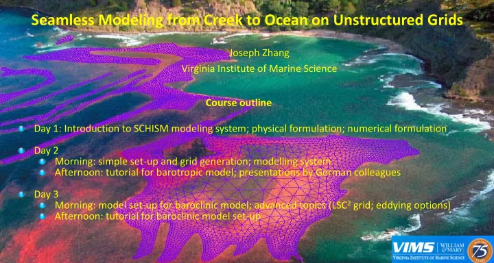
Seamless Modeling from Creek to Ocean on Unstructured Grids Joseph Zhang Virginia Institute of Marine Science Course outline Day 1: Introduction to SCHISM modeling system; physical formulation; numerical formulation Day 2 Morning: simple set-up and grid generation; modelling system Afternoon: tutorial for barotropic model; presentations by German colleagues Day 3 Morning: model set-up for baroclinic model; advanced topics (LSC 2 grid; eddying options) Afternoon: tutorial for baroclinic model set-up 1

Introduction to seamless cross-scale modeling: go small, go big

Matter of scales in GFD (Geophysical Fluid Dynamics) Most GFD processes are multi-scale in nature 3 c/o: Luke van Roeke

The messy reality of fish Dam(n)! • Fish migration respects no border/boundary • Best to be modeled using a large domain that encompasses the entire pathway 4

The great disappearing act of UG models 500m Storm surge (Westerink et al. 2008) Tsunami Grays Harbor UG models: “complex geometry, simple flow” Columbia River 500m SG models: “simple geometry, complex flow” 50km Baroclinic circulation is still mostly done using SG models with grid nesting Can we build a 500m baroclinic unstructured-grid (Oey et al. 2013) UG models are ‘natural’ for multi -scale model from river to ocean? processes…. Coos Bay but so far are mostly used for barotropic processes 5

Progress in the large- scale UG modeling…  MPAS o on Spherical Centroidal Voronoi Tessellations (SCVT), Arakawa-C grid (orthogonal), global o FV formulation (vector invariant) o Mostly free of spurious numerical ‘modes’ o Ocean, seaice, landice , atmosphere…  FESOM2 o on hybrid triangle-quads o FV formulation  ICON o on orthogonal triangles o FV formulation  However, significant challenges remain from deep ocean into shallow waters o Part of these challenges are due to physics (e.g., scale Skamarock et al. (2012) differences =>different parameterizations) o Scale-aware parameterization is an active research area o However, underlying numerics are lacking even if we restrict ourselves to hydrostatic regime 6

Sister model, MPAS-OI: a nearshore component of global MPAS-Ocean  Funded by US Dept. of Energy to bridge the gap between global ocean model and rivers o Both SCHISM and MPAS-OI will be fully coupled to MPAS-O  Formulation based on the subgrid, FV solver of UnTRIM (Casulli 2009), but with MPAS’ approach for conservation of mass, energy and potential vorticity (Thuburn et al. 2009)  The core is a semi-implicit, nonlinear solver for coupled continuity and momentum equation o The convergence of the nonlinear solver is always guaranteed o Enables mass conservative wetting and drying with any time step used  Subgrid capability for better representation of bathymetry

MPAS-OI: inundation test on a parabolic bowl Volume ratio Analytical Rotated symmetric bowl to test robustness Days

Seamless cross-scale modeling with SCHISM San Francisco Bay & Delta 9

Seamless cross-scale modeling with SCHISM • Bridge crossings on James River, Chesapeake Bay • Bridge pilings of 1-2m in diameter • ~1840 pilings located in the middle of salt intrusion path 10

SCHISM: Semi-implicit Cross-scale Hydroscience Integrated System Model A derivative product of SELFE v3.1, distributed with open-source Apache v2 license Substantial differences now exist between the two models Free svn access to release branch for general public Galerkin finite-element and finite-volume approach: generic unstructured triangular grids ELCIRC (Zhang et al. 2005), UnTRIM (Casulli 1990; 2010), SUNTANS (Fringer 2006): finite-difference/volume SELFE approach  orthogonal grid Hydrostatic or non-hydrostatic options Semi-implicit time stepping: no mode splitting  large time step and no splitting errors Eulerian-Lagrangian method (ELM) for momentum advection  more efficiency & robustness Major differences from SELFE v3.1 Apache license SCHISM Mixed grids (tri-quads) LSC 2 vertical grid (Zhang et al. 2015) Eddying regime (Zhang et al. 2016) Implicit TVD transport ( TVD 2 ) & WENO 3 Higher-order ELM with ELAD Bi-harmonic viscosity visit schism.wiki 11

c/o Karinna Nunez 12

Why SCHISM? Major differentiators from peer models No bathymetry smoothing or manipulation necessary: faithful representation of bathymetry is key in nearshore regime (Ye et al. 2018, OM) Implicit FE solvers  superior stability  very tolerant of bad-quality meshes (at least in non-eddying regime) Accurate yet efficient: implicit + low inherent numerical dissipation; flexible gridding system Need for grid nesting is minimized Well-benchmarked; certified inundation scheme for wetting and drying (NTHMP) Fully parallelized with domain decomposition (MPI+openMP) with strong scaling (via PETSc solver) Operationally tested and proven (DWR, EPA, NOAA, CWB …) Open source, with wider community support (210+ registered user groups) 13

Underlying numerics matter!  Explicit ‘mode - splitting’ models  Solves the hydrostatic equations in external and internal mode separately (splitting errors)  Easy to implement (with possible exception of filters), and well understood  99% of the existing models  Subject to CFL constraints (severe in shallow water)  Structured and unstructured grids  Excellent parallel scaling  Implicit models: the cross-scale models?  Solve the HS equations in one time step (no mode splitting errors)  Difficult to formulate (and parallelize)  No CFL constraints; superior stability  Mostly on unstructured grids  Parallel scaling not as good  Numerical diffusion needs to be carefully controlled UnTRIM SUNTANS ELCIRC In short, SCHISM is a very different type of beast from other ECOM-si SHYFEM conventional models, which has implications for usage! SELFE/SCHISM Unlearning prior experience with other models is required! 14

Underlying bathymetry matters even more : respect the bathymetry! Faithful representation of bathymetry is of fundamental importance especially in nearshore Two types of bathymetric errors Type I: Finite grid resolution; bathymetry survey errors; smoothing of DEM for unresolved sub-grid scales - not a convergence issue Type II: Smoothing or other manipulations (e.g. as in terrain-following coordinate models) - a divergence error as refining grid generally makes it worse! SCHISM’s representation of the bathymetry is piece -wise linear Very skew elements are allowed in non-eddying regime; implicit scheme guarantees stability Facilitates feature-tracking in grid generation There is no need for bathymetry smoothing to stabilize the model 15

Detrimental effects of bathymetry smoothing Smoothing in a critical region where the center Cross-channel transect with deep center channel channel constricts and bends, with multi-channel configurations Volume is conserved during smoothing 16 Ye et al. (2018)

Bathymetry smoothing effectively masks true numerical dissipation! Focusing on the cross transect on Smaller amplitude of tidal volume flux: The effect of smoothing on turbulent mixing: less the west part of the main stem, the smoothed = 79% original mixing overall and less contrast between shoal smoothing effects include: and channel Time averaged Vertical diffusivity [log 10 (m 2 s -1 )] Original More salt, about +1 PSU in the smoothed region, 2-3 PSU upstream Smoothed CB5.4 Larger sub-tidal volume flux 17 Ye et al. (2018)

Sensitivity test 1: mid-Bay smoothing Cross-sectional salinity distribution Less channel- shoal difference Original Smoothed Saltier bathymetry bathymetry 18

Sensitivity test 2: whole-Bay smoothing Stratification Channelized intrusion Uniform intrusion Original Smoothed Bathymetry Bathymetry More stratified due to stronger gravitational circulation 19

Sensitivity test 2: whole-Bay smoothing Salt budget (Lerczak et al., 2006) 𝐺 𝑡 ≈ 𝑅 𝑔 𝑡 0 + 𝐺 𝐹 + 𝐺 𝑈 𝑇 : total salt flux; 𝐺 𝐺 𝐹 : estuarine circulation flux; 𝐺 𝑈 : tidal oscillatory flux; 𝑅 𝑔 𝑡 0 : salt flux from river discharge and Stokes transport Transect 1 Transect 2 Transect 3 Larger salt flux due to estuarine circulation and Ye et al. (2018) tidal oscillation, leading to larger total flux 20

Grid generation in SCHISM: less numerics, more physics Tidal range Shoal Channel Skew elements Channel representation 21

How skew can you go?? Model is stable on very skew elements! 22

Extreme case #1: skew elements are a boon in nearshore applications Fringing marshes Smooth-transitioning grid would be 10x larger! In the non-eddying regime, skew elements can save a lot of computational cost! Fringing marshes need fine resolution (1m cross, 15m along) The implicit FE formulation in SCHISM makes it very tolerant of ‘bad’ meshes Fully coupled SCHISM-SED-WWM-Marsh model runs stably on this type of meshes Marsh migration in 30 years, with 4mm/yr sea-level rise Flow/wave impedance by marsh vegetation is incorporated in the implicit solver 23

Applications c/o: SCHISM users 16 1 2 3 4 10 12 1 2 16 11 4 13 13 8 9 12 15 7 5 5 3 14 6 11 8 15 6 9 14 7 10 24

San Francisco Bay & Delta  One of many success stories in SCHISM applications  Partnership with CA-DWR led to operational use of the model for drought and flood planning 25