Scientific Computing I Part I Module 5: Heat Transfer Discrete and - PDF document

Scientific Computing I Part I Module 5: Heat Transfer – Discrete and Contiuous Models Discrete Models Michael Bader Lehrstuhl Informatik V Winter 2006/2007 Motivation: Heat Transfer A Wiremesh Model consider rectangular plate as fine mesh of wires objective: compute the temperature distribution of compute temperature x ij at nodes of the mesh some object under certain prerequisites: temperature at object boundaries given x i,j+1 heat sources material parameters x i−1,j x i,j x i+1,j observation from physical experiments: x i,j−1 q ≈ k · δ T heat flow proportional to temperature differences 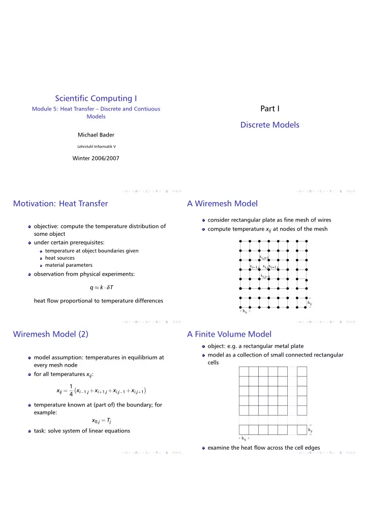h y h x Wiremesh Model (2) A Finite Volume Model object: e.g. a rectangular metal plate model as a collection of small connected rectangular model assumption: temperatures in equilibrium at cells every mesh node for all temperatures x ij : x ij = 1 � � x i − 1 , j + x i + 1 , j + x i , j − 1 + x i , j + 1 4 temperature known at (part of) the boundary; for example: x 0 , j = T j h y task: solve system of linear equations h x examine the heat flow across the cell edges

Heat Flow Across the Cell Boundaries Temperature change due to heat flow Heat flow across a given edge is proportional to temperature difference ( T 1 − T 0 ) between the in equilibrium: total heat flow equal to 0 adjacent cells but: consider additional source term F ij due to length h of the edge external heating e.g.: heat flow across the left edge: radiation q ( left ) F ij = f ij h x h y ( f ij heat flow per area) � � = k x T ij − T i − 1 , j h y ij equilibrium with source term requires q ij + F ij = 0: heat flow across all edges determines change of � � f ij h x h y = − k x h y 2 T ij − T i − 1 , j − T i + 1 , j heat energy: � � − k y h x 2 T ij − T i , j − 1 − T i , j + 1 q ij = k x � T ij − T i − 1 , j � h y + k x � T ij − T i + 1 , j � h y � � � � + k y T ij − T i , j − 1 h x + k y T ij − T i , j + 1 h x Finite Volume Model A Time Dependent Model divide by h x h y : − k x idea: set up ODE for each cell f ij = � 2 T ij − T i − 1 , j − T i + 1 , j � h x no external heat sources or drains: f ij = 0 − k y � � change of temperature per time is proportional to 2 T ij − T i , j − 1 − T i , j + 1 h y heat flow into the cell (no longer 0): again, system of linear equations κ x ˙ � � T ij ( t ) = 2 T ij ( t ) − T i − 1 , j ( t ) − T i + 1 , j ( t ) how to treat boundaries? h x κ y prescribe temperature in a cell � � + 2 T ij ( t ) − T i , j − 1 ( t ) − T i , j + 1 ( t ) h y (e.g. boundary layer of cells) prescribe heat flow across an edge; solve system of ODE for example insulation at left edge: q ( left ) = 0 ij From Discrete to Contiuous remember the discrete model: − k x � � f ij = 2 T ij − T i − 1 , j − T i + 1 , j Part II h x − k y � 2 T ij − T i , j − 1 − T i , j + 1 � A Continuous Model – The Heat h y Equation assumption:heat flow accross edges is proportional to temperature difference q ( left ) � � = k x T ij − T i − 1 , j h y ij in reality: heat flow proportional to temperature gradient T ij − T i − 1 , j q ( left ) ≈ kh y ij h x

From Discrete to Contiuous (2) Derivation of the Heat Equation replace k x by k / h x , k y by k / h y , and get: finite volume model, but with arbitrary control − k volume D � � f ij = 2 T ij − T i − 1 , j − T i + 1 , j h 2 change of heat energy (per time) is a result of x − k transfer of heat energy across D ’s surface, � � 2 T ij − T i , j − 1 − T i , j + 1 h 2 heat sources and drains in D (external influences) y resulting integral equation: consider arbitrary small cells: h x , h y → 0: ∂ � � � � ∂ 2 T � ∂ 2 T k ∇ T · � � � ρ cT dV = qdV + ndS f ij = − k − k ∂ t ∂ x 2 ∂ y 2 D D ij ij ∂ D leads to partial differential equation (PDE): density ρ , specific heat c , and heat conductivity k are material parameters � ∂ 2 T ( x , y ) + ∂ 2 T ( x , y ) � − k = f ( x , y ) heat sources and drains are modelled in term q ∂ x 2 ∂ y 2 Derivation of the Heat Equation (2) Heat Equations according to theorem of Gauß: Different scenarios: � � vanishing external influence, q = 0: k ∇ T · � ndS = k ∆ T dV D ∂ D T t = κ ∆ T leads to integral equation for any domain D : alternate notation � ρ cT t − q − k ∆ T dV = 0 � ∂ 2 T ∂ x 2 + ∂ 2 T ∂ y 2 + ∂ 2 T ∂ T � D ∂ t = κ · ∂ z 2 hence, the integrand has to be identically 0: equilibrium solution, T t = 0: T t = κ ∆ T + q κ := k ρ c , ρ c 0 = κ ∆ T + q − ∆ T = f − → ρ c κ > 0 is called the thermal diffusion coefficient (since the Laplace operator models a (heat) diffusion “Poisson’s Equation” process) Boundary Conditions Dirichlet boundary conditions: fix T on (part of) the boundary T ( x , y , z ) = ϕ ( x , y , z ) Neumann boundary conditions: fix T ’s normal derivative on (part of) the boundary: ∂ T ∂ n ( x , y , z ) = ϕ ( x , y , z ) special case: insulation ∂ T ∂ n ( x , y , z ) = 0