Scientific Computing I Part I Module 4: Numerical Methods for ODE - - PDF document

Scientific Computing I

Module 4: Numerical Methods for ODE Michael Bader

Lehrstuhl Informatik V

Winter 2005/2006

Part I Basic Numerical Methods Motivation: Direction Fields

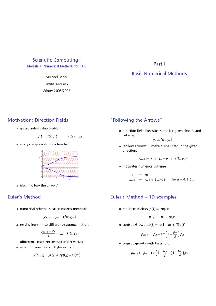
given: initial value problem: ˙ y(t) = f(t,y(t)), y(t0) = y0 easily computable: direction field

p(t) t 5 10 4 3 8 2 1 6 4 2

idea: “follow the arrows”

“Following the Arrows”

direction field illustrates slope for given time tn and value yn: ˙ yn = f(tn,yn) “follow arrows” = make a small step in the given direction: yn+1 := yn +τ ˙ yn = yn +τ f(tn,yn) motivates numerical scheme: y0 := y0 yn+1 := yn +τ f(tn,yn) for n = 0,1,2,...

Euler’s Method

numerical scheme is called Euler’s method: yn+1 := yn +τ f(tn,yn) results from finite difference approximation: yn+1 −yn τ ≈ ˙ yn = f(tn,yn) (difference quotient instead of derivative)

• r from truncation of Taylor expansion:

y(tn+1) = y(tn)+τ ˙ y(tn)+O(τ2)

Euler’s Method – 1D examples

model of Maltus, ˙ p(t) = αp(t): pn+1 := pn +τα pn Logistic Growth, ˙ p(t) = α (1−p(t)/β)p(t): pn+1 := pn +τα

• 1− pn

β

• pn

Logistic growth with threshold: pn+1 := pn +τα

• 1− pn

β

• 1− pn

δ

• pn

Euler’s Method in 2D

Euler’s method is easily extend to systems of ODE: yn+1 := yn +τ f(tn,yn) example: nonlinear extinction model ˙ p(t) =

• 71

8 − 23 12p(t)− 25 12q(t)

• p(t)

˙ q(t) =

• 73

8 − 25 12p(t)− 23 12q(t)

• q(t)

Euler’s method: ˙ p(t) = pn +τ

• 71

8 − 23 12pn − 25 12qn

• pn

˙ q(t) = qn +τ

• 73

8 − 25 12pn − 23 12qn

• qn

Discretized Model vs. Discrete Model

simplest example: model of Maltus pn+1 := pn −τα pn, α > 0 compare to discrete model: pn+1 := pn −δpn, δ > 0 with decay rate δ (“percentage”)

• bvious restriction in the discrete model: δ < 1
• bvious restriction for τ in the discretized model?

τα < 1 ⇒ τ < α−1 not that simple in non-linear models or systems of ODE!

Implicit Euler

Euler’s method (“explicit Euler”): yn+1 := yn +τ f(tn,yn) implicit Euler: yn+1 := yn +τ f(tn+1,yn+1) explicit formula for yn+1 not immediately available to do: solve equation for yn+1

Implicit Euler – Examples

example: Model of Maltus pn+1 := pn +τα pn+1 ⇒ pn+1 = 1 1−τα pn correct (discrete) model? α < 0 : then 0 < (1−τα)−1 < 1 for any τ α > 0 : then τ < α−1 required! in physics α < 0 is more frequent! (damped systems, friction, . . . ) implicit schemes preferred when explicit schemes require very small τ

Implicit Euler – 2D Example

example: arms race pn+1 = b1 +a11pn+1 +a12qn+1 qn+1 = b2 +a21pn+1 +a22qn+1) solve linear system of equations: (1−a11)pn+1 −a12qn+1 = b1 −a21pn+1 +(1−a22)qn+1 = b2 (for each time step n)

Local Discretisation Error

local influence of using differences instead of derivatives example: Euler’s method l(τ) = max

[a,b]

• yt+τ −y(t)

τ −f(t,y(t))

• memory hook: insert exact solution y(t) into

yn+1 −yn τ − ˙ yn A numerical scheme is called consistent, if l(τ) → 0 for τ → 0

Global Discretisation Error

compare numerical solution with exact solution example: Euler’s method e(τ) = max

[a,b] {yk −y(tk)}

(y(t) the exact solution; yk the solution of the discretized equation) A numerical scheme is called convergent, if e(τ) → 0 for τ → 0

Order of Consistency/Convergence

A numerical scheme is called consistent of order p (p-th

• rder consistent), if

l(τ) = O(τp) A numerical scheme is called convergent of order p (p-th order convergent), if e(τ) = O(τp)

Part II Advanced Numerical Methods Runge-Kutta-Methods

1st idea: use additional evaluations of f, e.g.: yn+1 = g(yn,f(tn,yn),f(tn+1,yn+1))

• pen question: where to obtain yn+1), how to

choose g 2nd idea: numerical approximations for missing values of y: yn+1 ≈ yn +τf(tn,yn) ⇒ yn+1 = g

• yn,f(tn,yn),f(tn+1,yn +τf(tn,yn))
• Runge-Kutta-Methods of 2nd order

3rd idea: choose g such that order of consistency is maximal example: 2nd-order Runge-Kutta: yn+1 = yn + τ 2

• f(tn,yn)+f(tn+1,yn +τf(tn,yn))
• (“method of Heun”)

further example: modified Euler (also 2nd order) yn+1 = yn +τ f

• tn + τ

2,yn + τ 2f(tn,yn))

• Runge-Kutta-Method of 4th order

classical 4th-order Runge-Kutta: intermediate steps: k1 = f(tn,yn) k2 = f

• tn + τ

2,yn + τ 2k1

• k3

= f

• tn + τ

2,yn + τ 2k2

• k3

= f (tn +τ,yn +τk3) explicit scheme: yn+1 = yn + τ 6

• k1 +2k2 +2k3 +k4

Multistep Methods

1st idea: use previous steps for computation: yn+1 = g(yn,yn−1,...,yn−q+1) 2nd idea: use integral form of ODE ˙ y(t) = f(t,y(t))

tn+1

• tn

˙ y(t)dt =

tn+1

• tn

f(t,y(t))dt y(tn+1)−y(tn) =

tn+1

• tn

f(t,y(t))dt =?

Multistep and Numerical Quadrature

3rd idea: use numerical method for integration → interpolate f using a polynomial p: y(tn+1)−y(tn) =

tn+1

• tn

f(t,y(t))dt ≈

tn+1

• tn

p(t)dt where p(tj) = f(tj,y(tj)) for j = n−s+1,...,n. compute integral and obtain quadrature rule: yn+1 = yn +

n

∑

j=n−s+1

αj f(tj,yj)

Adams-Bashforth

s = 1 ⇒ use yn only (leads to Euler’s method): p(t) = f(tn,yn), yn+1 = yn +τ f(tn,yn) s = 2 ⇒ use yn−1 and yn: p(t) = tn −t τ f(tn−1,yn−1)+ t−tn−1 τ f(tn,yn), yn+1 = yn + τ 2

• 3f(tn,yn)−f(tn−1,yn−1)
• usually consistent of s-th order

modified at start (no previous values available)

Adams-Moulton

use idea of Adams-Bashforth, but: include value yn+1 ⇒ implicit scheme first order: implicit Euler p(t) = f(tn+1,yn+1), yn+1 = yn +τ f(tn+1,yn+1) second order: yn+1 = yn + τ 2 (f(tn,yn)+f(tn+1,yn+1)) how to obtain yk+1?

solve (nonlinear) equation ⇒ difficult! easier and more common: predictor-corrector approach

Problems for Numerical Methods for ODE

Possible problems: Ill-Conditioned Problems: small changes in the input ⇒ big changes in the exact solution of the ODE Instability: big errors in the numerical solution compared to the exact solution (for arbitrarily small time steps although the method is consistent) Stiffness: small time steps required for acceptable errors in the approximate solution (although the exact solution is smooth)

Ill-Conditioned Problems

small changes in input entail completely different results Numerical treatment of such problems is always difficult! discriminate:

• nly at critical points?

everywhere?

possible risks:

non-precise input round-off errors,. . .

question: what are you interested in?

really the solution for specific initial condition? statistical info on the solution? general behaviour (patterns)?

Stability

Example: ˙ y(t) = −2y(t)+1, y(0) = 1 exact solution: y(t) = 1

2(e−2t +1)

well-conditioned: yε(0) = 1+ε ⇒ yε(t)−y(t) = εe−2t use midpoint rule (multistep scheme): yn+1 = yn−1 +2τ ·f(xn,yn) leads to numerical scheme: yn+1 = yn−1 +2τ (1−2yn)

Stability (2)

Observation: 2-step rule: yn+1 = yn−1 +2τ (1−2yn) start with exact initial values: y0 = y(0) and y1 = y(τ) numerical results for different sizes of τ:

τ = 1.0 ⇒ y9 = −4945.5, y10 = 20953.9 τ = 0.1 ⇒ y79 = −1725.3, y80 = 2105.7 τ = 0.01 ⇒ y999 = −154.6, y1000 = 158.7

midpoint rule is 2nd-order consistent, but does not converge here: oscillations or instable behaviour

Stability (3)

reason: difference equation generates spurious solutions analysis: roots µi of characteristic polynomial y2 = y0 +4τ(1−y); all |µi| < 1? Stability of ODE schemes: single step schemes: always stable multistep schemes: additional stability conditions in general: consistency + stability = convergence

Stiff Equations

Example: ˙ y(t) = −1000y(t)+1000, y(0) = y0 = 2 exact solution: y(t) = e−1000t +1 explicit Euler (stable): yk+1 = yk +τ(−1000yk +1000) = (1−1000τ)yk +1000τ = (1−1000τ)k+1 +1

• scillations and divergence for δt > 0.002

Why that? Consistency and stability are asymptotic terms!

Stiff Equations – Summary

Typical situation:

• ne term in the ODE demands very small time step

but does not contribute much to the solution Remedy: use implicit (or semi-implicit) methods

Summary

Runge-Kutta-methods: multiple evaluations of f (expensive, if f is expensive to compute) stable, well-behaved, easy to implement Multistep methods: higher order, but only evaluations of f (interesting, if f is expensive to compute) stability problems; behave “like wild horses” in practice: do not use uniform τ and s Implicit methods: for stiff equations most often used as corrector scheme