Scheduling MIMD parallel program A number of tasks executing - - PDF document

SLIDE 1

1

Lecture 5: Load Balancing

2

Scheduling

• MIMD parallel program

– A number of tasks executing serially or in parallel

• The scheduling problem NP-complete problem (in general)

– Distribute tasks on processors so that minimal execution time is achieved

• Optimal distribution

– Processor allocation + execution order such that the execution time is minimized

• Scheduling system (Consumer, Policy, Resource)

Consumer Resource Scheduler Policy

3

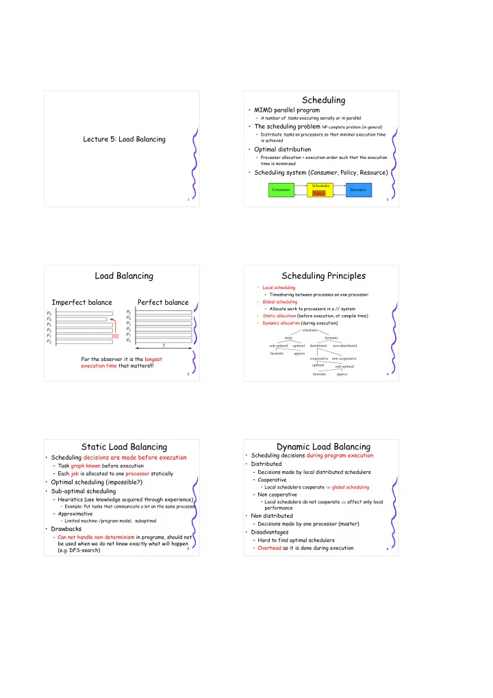
Load Balancing

Imperfect balance Perfect balance

For the observer it is the longest execution time that matters!!!

4

Scheduling Principles

• Local scheduling

– Timesharing between processes on one processor

• Global scheduling

– Allocate work to processors in a // system

• Static allocation (before execution, at compile time)
• Dynamic allocation (during execution)

scheduler static dynamic sub-optimal

• ptimal

heuristic approx distributed non-distributed cooperative non cooperative

• ptimal

sub-optimal approx heuristic 5

Static Load Balancing

• Scheduling decisions are made before execution

– Task graph known before execution – Each job is allocated to one processor statically

• Optimal scheduling (impossible?)
• Sub-optimal scheduling

– Heuristics (use knowledge acquired through experience)

• Example: Put tasks that communicate a lot on the same processor

– Approximative

• Limited machine-/program-model, suboptimal
• Drawbacks

– Can not handle non-determinism in programs, should not be used when we do not know exactly what will happen (e.g. DFS-search)

6

Dynamic Load Balancing

• Scheduling decisions during program execution
• Distributed

– Decisions made by local distributed schedulers – Cooperative

• Local schedulers cooperate ⇒ global scheduling

– Non cooperative

• Local schedulers do not cooperate ⇒ affect only local

performance

• Non distributed

– Decisions made by one processor (master)

• Disadvantages

– Hard to find optimal schedulers – Overhead as it is done during execution

SLIDE 2

7

Other kinds of scheduling

• Single application / multiple application system
• Only one application at the time, minimize execution time

for that application

• Several parallel applications (compare to batch-queues),

minimize the average execution time for all applications

• Adaptive / non adaptive scheduling
• Changes behavior depending on feedback from the system
• Is not affected by feedback
• Preemptive / non-preemptive scheduling
• Allows a process to be interrupted if it is allowed to

resume later on

• Does not allow a process to

be interrupted

1 3 2 2

preemptive non-preemptive

1 3

8

Static Scheduling

• Graph Theory Approach

– (for programs without loops and jumps) – DAG (directed acyclic graph) = task graph – Start-node (no parents), exit-node (no children)

• Machine Model

– Processors P = {P1, ..., Pm} – Edge matrix (mxm), comm-cost Pi,j – Processor performance Si [instructions per second]

• Parallel Program Model

– Tasks T = {T1, ..., Tn} – The execution order is given by the arrows – Communication matrix (nxn), no. elem. Di,j – Number of instructions Ai

1 5 3 5 5 5 4 8 2 10 1 1 2 2 2 3

T1, A1, D14

9

Construction of schedules

• Schedule: mapping that allocates one or more

disjunct time interval to each task so that – Exactly one processor gets each interval – The sum of the intervals equals the execution time for the task – Different intervals on the same processor do not overlap – The order between tasks is maintained – Some processor is always allocated a job

10

Optimal Scheduling Algorithms

• The scheduling problem is NP complete for the general
• case. Exceptions:

– HLF (Highest Level First), CP (Critical Path), LP (Longest Path) which in most cases gives optimal scheduling

• List scheduling: priority list with nodes and allocate the nodes
• ne by one to the processes. Choose the node with highest

priority and allocate that to the first available process. Repeat until the list is empty. – It varies between algorithms how to compute priority

• Tree structured task graph. Simplification:

– All tasks have the same execution time – All processors have the same performance

• Arbitrary task graph on two processors. Simplification:

– All tasks have the same execution time

11

List Scheduling

• Remember

– Each task is allocated a priority & is placed in a list sorted by priority – When a processor is free, allocate the task with the highest priority

• If two tasks have the same priority, take one randomly
• Different choice of priority gives different kinds of

scheduling

– Level gives closest to optimal priority order (HLF)

1 1 2 1 3 2

1

4 1

1 1 1 1 2 3 4 1 1 2 3 2 2 1

Task Level #Pr

Number of reasons I'm not ready

12

Scheduling of a tree structured task graph

• Level

– maximum number of nodes from x to a terminal node

• Optimal algorithm (HLF)

– Determine the level of each node = priority – When a processor is available, schedule the ready task with the highest priority

• HLF can fail

– You can always construct an example that fails – Works for most algorithms

SLIDE 3

13

Scheduling Heuristics

• The complexity increases if the model allows

– Tasks with different execution times – Different speed of the communication links – Communication conflicts – Loops and jumps – Limited networks

• Find suboptimal solutions

– Find, with the help of a heuristic, solutions that most of the time are close to optimal

14

Parallelism vs Communication Delay

• Scheduling must be based on both

– Communication delay – The time when a processor is ready to work

• Trade-off between maximizing the parallelism &

minimizing the communication (max-min problem)

1 2 3 Dx

P1 P2

1 2 3 3 Dx Dx > T2

P1 P2

1 2 3 Dx Dx < T2

15

Example, Trade-off // vs Communication Time

D3 < T2, assign T3 to P2 Time = T1 + D3 + T3 + Dy + T4 , or Time = T1 + T2 + Dx + T4 If min(Dx, Dy) > T3 assign T3 to P1

P1 P2

1 2 3 D3 4 Dy

P1 P2

1 2 3 D3 Dx 4 1 2 3 4

P1

1 2 3 D3 4 D2 Dy Dx

16

The Granularity Problem

• Find the best clustering of tasks in the task

graph (minimize execution time)

• Coarse Grain

– Less parallelism

• Fine Grain

– More parallelism – More scheduling time – More communication conflicts

17

Redundant Computing

• Sometimes you may eliminate communication delays

by duplicating work

1 1 2 1 3 1

1

4 1

1 1 1 1 2 4

P1 5 1

1 1 3 5

P2

1 2 4

P1

3 3

P2

5

18

Dynamic Load Balancing

• Local scheduling

Example: Threads, Processes, I/O

• Global scheduling

Example: Some simulations – Pool of tasks / distributed pool of tasks

• receiver-initiated or sender-initiated

– Queue line structure

SLIDE 4

19

Pool of Tasks

• Centralized
• Decentralized
• Distributed
• How to choose processor

to communicate with?

Centralized Decentralized Distributed 20

Work Transfer - Distributed

• The receiver takes the initiative. ”Pull”

– One process asks another process for work – The process asks when it is out of work, or has too little to do. – Works well, even when the system load is high – Can be expensive to approximate system loads

21

Work Transfer - Distributed

• The sender takes the initiative. ”Push”

– One process sends work to another process – The process asks (or just sends) when it has too many tasks, or high load – Works well when the system load is low – Hard to know when to send

22

Work Transfer - Decentralized

• Example of

process choices – Load

• (hard)

– Round robin

• Must make sure that the

processes do not “get in phase”, i.e. they all ask the same process – Randomly (random polling)

• Good generator necessary??

23

Queue Line Structure

• Have two processes per node
• One worker process that

– computes – asks the queue for work

• Another that

– asks (to the left) for new tasks if the queue is nearly empty – receives new tasks from the left neighbor – receives requests from the right neighbor and from the worker process and answers these requests

24

Tree Based Queue

• Each process sends to one of two processes

– generalization of the previous technique

SLIDE 5

25

Example – Shortest Path

• ”Given a set of linked nodes where the

edges between the nodes are marked with ’weights’, find the path from one specific node to another that has the least accumulated weight.”

• How do you represent the graph?

26

Example – Shortest Path

27

Moore's Algorithm

• dj=min(dj, di+wi,j)
• Keep a queue, containing vertices not yet

computed on. Begin with the start vertex.

• Keep a list with shortest distances. Begin with

zero for the start vertex, and infinity for the

• thers.
• For each node in the beginning of the queue,

update the list according to the expression

• above. If there is an update, add the vertex to

the queue again.

28

Sequential code

• Using an adjacency matrix.

while ((i = next_vertex()) != no_vertex) /* while a vertex */ for (j = 1; j < n; j++) /* get next edge */ if (w[i][j] != infinity) { /* if an edge */ newdist_j = dist[i] + w[i][j]; if (newdist_j < dist[j]) { dist[j] = newdist_j; append_queue(j); /* vertex to queue if not there */ } } /* no more vertices to consider */

29

Parallel Implementation I

• Dynamic load balancing
• Centralized work pool

– Each computational node takes vertices from the queue and returns new vertices – The distances are stored as a list, copied

• ut to the nodes

30

Parallel Implementation I

• Code:

while (vertex_queue() != empty) { recv(PANY, source = Pi); v = get_vertex_queue(); send(&v, Pi); send(&dist, &n, Pi); . recv(&j, &dist[j], PANY, source = Pi); append_queue(j, dist[j]); }; recv(PANY, source = Pi); send(Pi, termination_tag); While(true){ send(Pmaster); recv(&v, Pmaster, tag); if (tag != termination_tag) { recv(&dist, &n, Pmaster); for (j = 1; j < n; j++){ if (w[v][j] != infinity) { newdist_j = dist[v] + w[v][j]; if (newdist_j < dist[j]) { dist[j] = newdist_j; send(&j, &dist[j], Pmaster); } } } } else {break;} }

SLIDE 6

31

Parallel Implementation II

• Decentralized work pool

– Each vertex is a process. As soon as a vertex gets a new weight (start node → it self), it sends new distances to its neighbors

32

Parallel Implementation – II

• Code:

recv(newdist, PANY); if (newdist < dist) dist = newdist; /* start searching around vertex */ for (j = 1; j < n; j++) /* get next edge */ if (w[j] != infinity) { d = dist + w[j]; send(&d, Pj); /* send distance to proc j */ }

• Have to handel ”messages in the air”.

(MPI_Probe)

33

Shortest Path

• Probably have to group the vertices, i.e., several

vertices per processor.

• Vertices close to each other on the same processor ⇒

– Little communication – Little parallelism

• Vertices far away on the same processor (scatter) ⇒

– Lot of communication – Much parallelism – Group messeges? Synchronizing?

• Terminating

34

Terminating Algorithms

Ring algorithm:

• Let a process p0 send a token on

the ring when p0 is out of work

• When a process receives a token:

– If out of work, pass the token on – If not, wait until out of work, and then pass the token on

• When p0 gets back the token, p0

knows that everyone is out of work

• Can notify the others
• Does not work if processes

”borrows” work from each other p0

35

Terminating Algorithms

Dijkstra's ring algorithm:

• Let a process p0 send a white token on the ring

when p0 is out of work

• If a process pi sends work to pj, j < i, it will be

colored black

• When a process receives a token:

– If the process is black, the token is colored black – If out of work, pass the token on – If not, wait until out of work, then pass the token on

• If p0 gets a white token back, p0 knows that

everyone is out of work – sends a terminating message (e.g., a red token)

• If p0 gets a black token back, p0 sends out a white

token

pj p0 pi

work

36

Kontrollfrågor

• Antag att fem (arbets-)processer ska

lösa shortest path för grafen till höger med ”Parallell implementation I”. Hur många, och vilka, meddelanden skickas?

• Antag att fem (arbets-)processer ska

lösa shortest path för grafen till höger med ”Parallell implementation II”. Hur många, och vilka, meddelanden skickas?

• Hitta en optimal tidsfördelning för task-

grafen till höger för två processorer.

1 2 3 4 5 2 3 7 3 5 12 2 2 1 10