Module 5: CPU Scheduling Basic Concepts Scheduling Criteria - - PDF document

Module 5: CPU Scheduling

• Basic Concepts
• Scheduling Criteria
• Scheduling Algorithms
• Multiple-Processor Scheduling
• Real-Time Scheduling
• Algorithm Evaluation

Operating System Concepts 5.1 Silberschatz and Galvin c 1998

Basic Concepts

• Maximum CPU utilization obtained with multiprogramming.
• CPU–I/O Burst Cycle – Process execution consists of a cycle of

CPU execution and I/O wait.

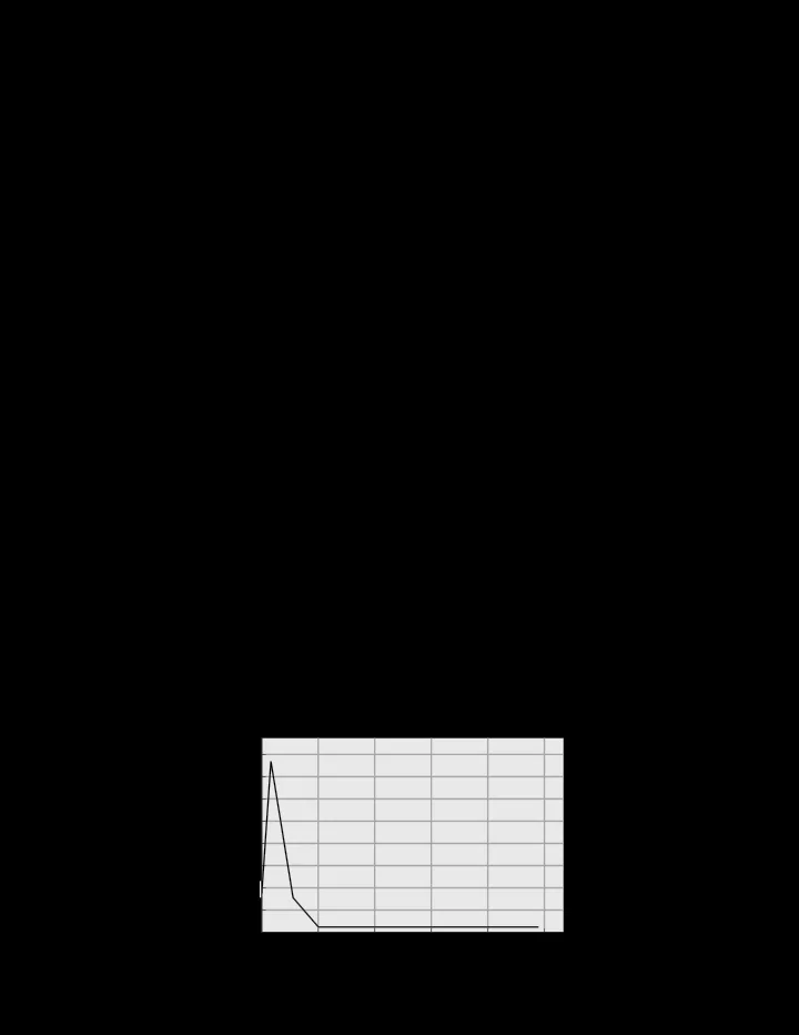
• CPU burst distribution

burst duration (milliseconds) frequency 20 40 60 80 100 120 140 160 8 16 24 32 40 Operating System Concepts 5.2 Silberschatz and Galvin c 1998

CPU Scheduler

• Selects from among the processes in memory that are ready to

execute, and allocates the CPU to one of them.

• CPU scheduling decisions may take place when a process:
• 1. switches from running to waiting state.
• 2. switches from running to ready state.
• 3. switches from waiting to ready.
• 4. terminates.
• Scheduling under 1 and 4 is nonpreemptive.
• All other scheduling is preemptive.

Operating System Concepts 5.3 Silberschatz and Galvin c 1998

Dispatcher

• Dispatcher module gives control of the CPU to the process

selected by the short-term scheduler; this involves: – switching context – switching to user mode – jumping to the proper location in the user program to restart that program

• Dispatch latency – time it takes for the dispatcher to stop one

process and start another running.

Operating System Concepts 5.4 Silberschatz and Galvin c 1998

Scheduling Criteria

• CPU utilization – keep the CPU as busy as possible
• Throughput – # of processes that complete their execution per

time unit

• Turnaround time – amount of time to execute a particular

process

• Waiting time – amount of time a process has been waiting in

the ready queue

• Response time – amount of time it takes from when a request

was submitted until the first response is produced, not output (for time-sharing environment)

Operating System Concepts 5.5 Silberschatz and Galvin c 1998

Optimization Criteria

• Max CPU utilization
• Max throughput
• Min turnaround time
• Min waiting time
• Min response time

Operating System Concepts 5.6 Silberschatz and Galvin c 1998

First-Come, First-Served (FCFS) Scheduling

• Example:

Process Burst Time P1 24 P2 3 P3 3

• Suppose that the processes arrive in the order: P1, P2, P3

The Gantt chart for the schedule is:

P1 P

2

P

3

30 27 24

• Waiting time for P1 = 0; P2 = 24; P3 = 27
• Average waiting time:

(0 + 24 + 27)/3 = 17

Operating System Concepts 5.7 Silberschatz and Galvin c 1998

FCFS Scheduling (Cont.)

Suppose that the processes arrive in the order: P2, P3, P1.

• The Gantt chart for the schedule is:

P1 P

2

P

3

3 6 30

• Waiting time for P1 = 6; P2 = 0; P3 = 3
• Average waiting time:

(6 + 0 + 3)/3 = 3

• Much better than previous case.
• Convoy effect: short process behind long process

Operating System Concepts 5.8 Silberschatz and Galvin c 1998

Shortest-Job-First (SJF) Scheduling

• Associate with each process the length of its next CPU burst.

Use these lengths to schedule the process with the shortest time.

• Two schemes:

– nonpreemptive – once CPU given to the process it cannot be preempted until it completes its CPU burst. – preemptive – if a new process arrives with CPU burst length less than remaining time of current executing process,

• preempt. This scheme is known as the

Shortest-Remaining-Time-First (SRTF).

• SJF is optimal – gives minimum average waiting time for a

given set of processes.

Operating System Concepts 5.9 Silberschatz and Galvin c 1998

Example of Non-Preemptive SJF

Process Arrival Time Burst Time P1 0.0 7 P2 0.2 4 P3 4.0 1 P4 5.0 4

• SJF (non-preemptive)

P1 P

3

P

2

P

4

16 7 8 12

Average waiting time = (0 + 6 + 3 + 7)/4 = 4

Operating System Concepts 5.10 Silberschatz and Galvin c 1998

Example of Preemptive SJF

Process Arrival Time Burst Time P1 0.0 7 P2 0.2 4 P3 4.0 1 P4 5.0 4

• SRTF (preemptive)

P

2

P

2

P

3

P1 P

4

P1 11 16 7 5 4 2

Average waiting time = (9 + 1 + 0 + 2)/4 = 3

Operating System Concepts 5.11 Silberschatz and Galvin c 1998

Determining Length of Next CPU Burst

• Can only estimate the length.
• Can be done by using the length of previous CPU bursts, using

exponential averaging.

• 1. tn = actual length of nth CPU burst
• 2. τn+1 = predicted value for the next CPU burst
• 3. α, 0 ≤ α ≤ 1
• 4. Define:

τn+1 = α tn + (1 − α)τn.

Operating System Concepts 5.12 Silberschatz and Galvin c 1998

Examples of Exponential Averaging

• α = 0

– τn+1 = τn – Recent history does not count.

• α = 1

– τn+1 = tn – Only the actual last CPU burst counts.

• If we expand the formula, we get:

τn+1 = αtn + (1 − α)αtn−1 + ... +(1 − α)jαtn−j + ... +(1 − α)n+1τ0

• Since both α and (1 − α) are less than or equal to 1, each

successive term has less weight than its predecessor.

Operating System Concepts 5.13 Silberschatz and Galvin c 1998

Priority Scheduling

• A priority number (integer) is associated with each process.
• The CPU is allocated to the process with the highest priority

(smallest integer ≡ highest priority). – preemptive – nonpreemptive

• SJN is a priority scheduling where priority is the predicted next

CPU burst time.

• Problem ≡ Starvation – low priority processes may never

execute.

• Solution ≡ Aging – as time progresses increase the priority of

the process.

Operating System Concepts 5.14 Silberschatz and Galvin c 1998

Round Robin (RR)

• Each process gets a small unit of CPU time (time quantum),

usually 10–100 milliseconds. After this time has elapsed, the process is preempted and added to the end of the ready queue.

• If there are n processes in the ready queue and the time

quantum is q, then each process gets 1/n of the CPU time in chunks of at most q time units at once. No process waits more than (n − 1)q time units.

• Performance

– q large ⇒ FIFO – q small ⇒ q must be large with respect to context switch,

• therwise overhead is too high.

Operating System Concepts 5.15 Silberschatz and Galvin c 1998

Example: RR with Time Quantum = 20

Process Burst Time P1 53 P2 17 P3 68 P4 24

• The Gantt chart is:

P

2

P1 P

3

P

4

P1 P

3

P

4

P1 P

3

P

3

162 154 134 121 117 97 77 57 37 20

• Typically, higher average turnaround than SRTF, but better

response.

Operating System Concepts 5.16 Silberschatz and Galvin c 1998

Multilevel Queue

• Ready queue is partitioned into separate queues;

foreground (interactive) background (batch)

• Each queue has its own scheduling algorithm,

foreground – RR background – FCFS

• Scheduling must be done between the queues.

– Fixed priority scheduling; i.e., serve all from foreground then from background. Possibility of starvation. – Time slice – each queue gets a certain amount of CPU time which it can schedule amongst its processes; i.e., 80% to foreground in RR 20% to background in FCFS

Operating System Concepts 5.17 Silberschatz and Galvin c 1998

Multilevel Feedback Queue

• A process can move between the various queues; aging can

be implemented this way.

• Multilevel-feedback-queue scheduler defined by the following

parameters: – number of queues – scheduling algorithm for each queue – method used to determine when to upgrade a process – method used to determine when to demote a process – method used to determine which queue a process will enter when that process needs service

Operating System Concepts 5.18 Silberschatz and Galvin c 1998

Example of Multilevel Feedback Queue

• Three queues:

– Q0 – time quantum 8 milliseconds – Q1 – time quantum 16 milliseconds – Q2 – FCFS

• Scheduling

– A new job enters queue Q0 which is served FCFS. When it gains CPU, job receives 8 milliseconds. If it does not finish in 8 milliseconds, job is moved to queue Q1. – At Q1, job is again served FCFS and receives 16 additional

• milliseconds. If it still does not complete, it is preempted

and moved to queue Q2.

Operating System Concepts 5.19 Silberschatz and Galvin c 1998

Multiple-Processor Scheduling

• CPU scheduling more complex when multiple CPUs are

available.

• Homogeneous processors within a multiprocessor.
• Load sharing
• Asymmetric multiprocessing – only one processor accesses

the system data structures, alleviating the need for data sharing.

Operating System Concepts 5.20 Silberschatz and Galvin c 1998

Real-Time Scheduling

• Hard real-time systems – required to complete a critical task

within a guaranteed amount of time.

• Soft real-time computing – requires that critical processes

receive priority over less fortunate ones.

Operating System Concepts 5.21 Silberschatz and Galvin c 1998

Algorithm Evaluation

• Deterministic modeling – takes a particular predetermined

workload and defines the performance of each algorithm for that workload.

• Queueing models
• Implementation

Operating System Concepts 5.22 Silberschatz and Galvin c 1998