
SLIDE 1
CPU Scheduling
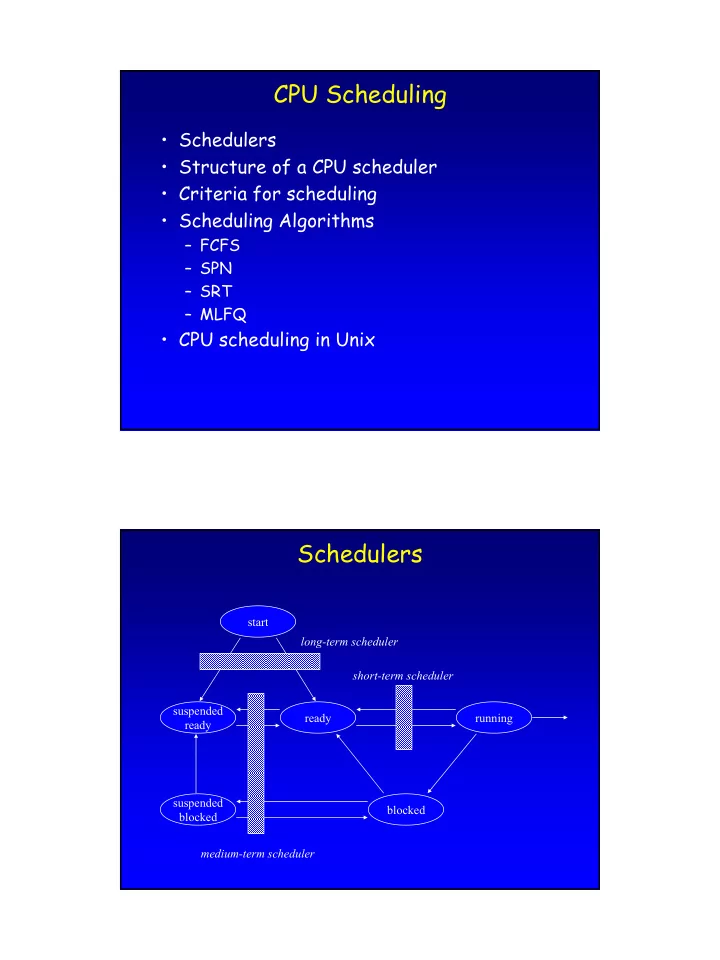
- Schedulers
- Structure of a CPU scheduler
- Criteria for scheduling
- Scheduling Algorithms
– FCFS – SPN – SRT – MLFQ
- CPU scheduling in Unix