MIMD Multicomputer Mesh, ring, linear array, 2D-torus, 3D-mesh - - PDF document

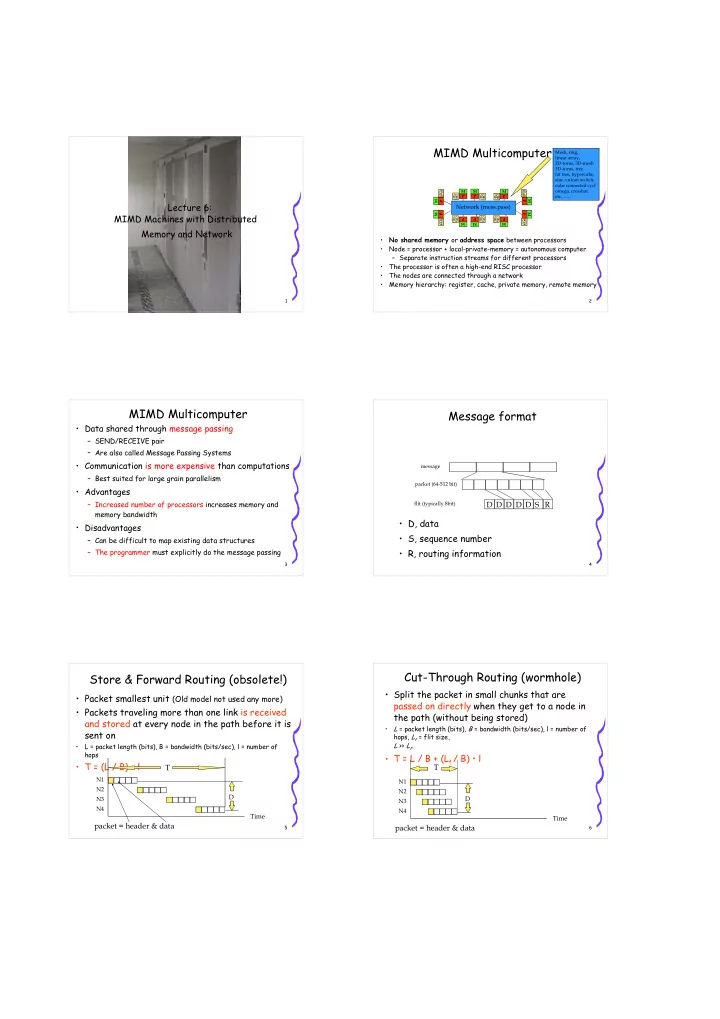
Lecture 6: MIMD Machines with Distributed Memory and Network

MIMD Multicomputer

• No shared memory or address space between processors
• Node = processor + local-private-memory = autonomous computer

– Separate instruction streams for different processors

• The processor is often a high-end RISC processor
• The nodes are connected through a network
• Memory hierarchy: register, cache, private memory, remote memory

• mega, crossbar,

Network (mess.pass)

MIMD Multicomputer

• Data shared through message passing

– SEND/RECEIVE pair – Are also called Message Passing Systems

• Communication is more expensive than computations

– Best suited for large grain parallelism

• Advantages

– Increased number of processors increases memory and memory bandwidth

• Disadvantages

– Can be difficult to map existing data structures – The programmer must explicitly do the message passing

Message format

• D, data
• S, sequence number
• R, routing information

packet (64-512 bit) message flit (typically 8bit)

R S D D D D D

Store & Forward Routing (obsolete!)

• Packet smallest unit (Old model not used any more)
• Packets traveling more than one link is received

and stored at every node in the path before it is sent on

• L = packet length (bits), B = bandwidth (bits/sec), l = number of

hops

• T = (L / B) • l

Time

N2 N1 N3 N4

T

D

packet = header & data

Cut-Through Routing (wormhole)

• Split the packet in small chunks that are

passed on directly when they get to a node in the path (without being stored)

• L = packet length (bits), B = bandwidth (bits/sec), l = number of

hops, Lf = flit size, L >> Lf.

• T = L / B + (Lf / B) • l

T

Time

N2 N1 N3 N4

D

packet = header & data

Example: Message Passing on the IBM SP

• The message is split in a number of packets

– the packet is split in a number of flits – one flit = 1 byte – the packets varies in length up to 255 flits – flit1 = packet length, flit2 - flitr = routing info, the rest is data – each switch step: checks the 1st route-flit, determines the “out- port”, removes the flit (when the packet has reached the destination it no longer contains any route-flits)

• Buffered Wormhole routing

– a flit is moved to the “out-port” as soon as it has arrived on the “in- port” – “the right” “out-port” is determined by the second flit in the packet – if links are busy, flits are stored in a for all “in-ports” shared buffer (central queue)

Message Passing Programming

• Formulate programs in terms of sending and

receiving messages

• Programs are portable between different

machines with small changes (e.g., IBM SP, cluster, network of work stations)

• To be able to exchange messages the nodes

have to know

• each others identity
• the size of the message
• content type of the message

Programming DMM systems

(SPMD-Single Program Multiple Data) program myfirst me = myid() npr = numprocs() x = rand() write(x,me) to = me+1 mod npr from = me+npr-1 mod npr send(x, to) receive(y,from) write(y,me) end

1 2

• 1. The same program is loaded on all nodes
• 2. Every node starts to execute its own copy of the program
• 3. Data is exchanged by send and receive pairs
• 4. Synchronizing

implicit by communication explicit by barriers

Execution of programs

program myfirst me = 0 npr = 3 x = 0.25 write(0.25, 0) to = 1 from = 2 send(0.25, 1) receive(y, 2) write(0.1, 0) end

1 2

program myfirst me = 1 npr = 3 x = 0.65 write(0.65, 1) to = 2 from = 0 send(0.65, 2) receive(y, 0) write(0.25, 1) end program myfirst me = 2 npr = 3 x = 0.1 write(0.1, 2) to = 0 from = 1 send(0.1, 0) receive(y, 1) write(0.65, 2) end

1 2

Communication

• Minimize communication overhead
• Communication cost for ”point-to-point”

Store-and-forward: tc = (α + βL) * #hops Cut-through: tc = α + βL ♦ α is the startup cost (”node latency”) and β is the cost per unit (usally bytes) per link ♦ α >> β ⇒

− α dominates for small messages − β dominates for large messages

Collective operations: broadcast, gather, scatter etc.

• Group messages whenever possible
• Use more than one copy of the data?
• Repeat identical computations/share the result?
• Overlapping computations/communication?

Network

The topology of a network can be either static

• r dynamic
• Statical Networks

– Point-to-point, direct connections – Does not change during program execution

• Dynamical Networks

– Switches – Dynamically configured to fit the needs of the program

Network Parameters

• Network size (N): number of nodes
• Node degree (d)

– number of links/channels on each node – one-way channels in/out degree, (node degree = in + out degree) – small node degree good, cheap and modular

• Network diameter (D)

– max(shortest path between two arbitrary nodes) – measured in number of links traversed (hops) – small diameter is good

• Bisection width (b)

– smallest number of edges between two halves of the network

Static Connected Networks

• Linear array

– N nodes, N-1 links – Inner nodes: node degree d = 2, outer nodes: node degree d = 1 – diameter D = N-1 – bisection width b = 1

• Ring, node degree d = 2

– N nodes, N links – diameter D = N (for bidirectional ring N/2) – bisection width b = 2

• Ring, node degree d = 3, Chorodal ring of degree 3

– Increase number of links, higher node degree and lower diameter

• Ring, node degree d = N-1 : Fully coupled network

– diameter D = 1

• Star (tree with two levels)

– degree d = N-1, diameter D = 2

• Fat tree

– more (fatter) channels closer to the root

Static Connected Networks

Mesh & Torus

• Mesh, k-dimensional with

N = nk nodes has

– node degree d = 2k for the inner nodes – diameter D = k(n-1) – Note! not symmetric; edge nodes has degree 2 or 3 (for k=2)

• Torus

– nxn mesh with wraparounds in row & column dimensions – symmetric

• d = 4
• D = 2n/2 = n

HPC2N Super Cluster –

seth.hpc2n.umu.se

• 240 processors i 120 dual nodes
• Nodes connected in a 4 x 5 x 6 mesh network

with “wrap arounds”

• Built by HPC2N (and CS)
• 12 racks
• Was build during April-May 2002
• Available for users 2002-06
• 83% usage (24h/day – 7 days/week) since

2002-08

• Total peak performance 800 Gflops/s
• Top500 2002-06:

– 94th fastest in the world – fastest in Sweden

• Financing: 5 MSEK from the Kempe

Foundations

SCI Network

• Wulfkit3 SCI network by Dolphin IS, Norway
• The nodes are connected in a 4 x 5 x 6 mesh network with

“wrap arounds”

• 667 Mbytes/s peak bandwidth => peak 1.43E-9 sec/byte
• 1.46 µsec node latency
• ScaMPI message passing library (MPI) from Scali AS
• Software for system surveillance and system management

Seth - Pallas MPI Benchmark

(Multi(16) is pairwise ping-pong between 8 pairs of processors) 230 Mbytes/s max bandwidth 3.7 µsec minimum latency

Static Connected Networks Hypercube

When the distance along one axis is indicated by a binary number, the hypercube is called binary

• Binary n-cube

– Hypercube of/with dimension n

• N = 2n (n = log2 N)

– node degree d = dimension = diameter D = n – Number of links d•N/2 – The nodes are numbered from 0 to 2d- 1 – Many other architectures can be mapped on a HC (embedding)

• linear array, ring, tree, mesh

– Many algorithms are adapted for HC – often very effective

Hypercube

• Two nodes are nearest neighbors if only one bit

differs in the binary representation

• ”The Hamming distance” between two binary

numbers are the bits differing (xor) – is e.g., used to find the path between two nodes

Making a cube of dimension d starting from a cube of dimension d-1

1) make a copy of the d-1 cube 2) draw edges between the original and the copy 3) put a 0 in front of the binary code of the original 4) put a 1 in front of the copy 1

• riginal

d = 1 Step 1 2 3 4 1 1 00 01 1 00 01 10 11 1 1 new HC d = 2

Partitioning a Hypercube

• Partitioning a d-dim. cube into two d-1 dim cubes

– choose a bit position in the binary code and group every node with a 0 in that position, all these form a subcube. The ones with a 1 in that position forms another subcube

• Partition a d-dim cube into 2k subcubes

– fix k positions in the binary code and let these form subcubes

Binary Reflected Gray Code

• Binary Reflected Gray Code, RGC, is used

to map other structures on a HC – d-bit binary gray code – S1 = 0, 1 – Sk = 0[Sk-1], 1[Sk-1]R (R = reflected) 00, 01, 11, 10 -R-> ( 10, 11, 01, 00 ) 000, 001, 011, 010, 110, 111, 101, 100

• G(i, d) = i:th component in a d-bit Gray code

sequence (i=0,1,2...)

• G(3,3) = 010

0000 0001 0011 0010 0110 0111 0101 0100 1100 1101 1111 1110 1010 1011 1001 1000

Binary Reflected Gray Code

• The function G(i,d) describes the mapping of node i on a linear

array/ring on a hypercube:

• G(i,d) also gives the i:th code in a sequence of d-bit Gray
• code. Gray code with d+1 bits is derived from a table of the

d-bit Gray code by reflecting the table and put a 0 in front of the original codes and a 1 in front of the reflected code.

• Note that G(i,d) och G(i+1,d) differs in exactly one bit

   ≥ − − + < = + = =

i x i G i x i G x i G G G 2 ), , 1 2 ( 2 2 ), , ( ) 1 , ( 1 ) 1 , 1 ( ) 1 , (

Mapping other networks on a Hypercube

• Linear Array on a HC

– processor i in the linear array is mapped on processor G(i, d) in the HC – Processor i is a (physical) nearest neighbor to i-1 and i+1

• Ring on a HC

– in the same way as a linear array – processor p-1 is processor a (physical) nearest neighbor to

• 2-D Torus on a HC

– Mapping a 2r x 2s torus on a 2r+s processor hypercube – node (i,j) in the mesh is mapped on G(i, r)||G(j, s) on the hypercube (||=concat) – Logical neighbors in the mesh will be physical neighbors on the cube

0000 0001 0011 0010 0110 0111 0101 0100 1100 1101 1111 1110 1010 1011 1001 1000

Example: map a ring/array on a hypercube

• 8 CPU (d = 3)
• Gray code, HC pid, Ring/Array pid

– 000 – 001 1 1 – 011 3 2 – 010 2 3 – 110 6 4 – 111 7 5 – 101 5 6 – 100 4 7

Message Passing Mechanisms Routing

• XY-routing in a 2-D Mesh:

– Step to the proper column on the x-axis, then on the y-axis to the destination – Minimal routing = |Sx -Dx| + |Sy - Dy|

• E-cube routing on a Hypercube:

– S and D are the starting point and destination – Both are represented by a d-bit string

• compute the Hamming Distance (S xor D)
• send along the channel pointed to by the least

significant 1 in the Hamming Distance

• name the reached node S and repeat the process

0000 0001 0011 0010 0110 0111 0101 0100 1100 1101 1111 1110 1010 1011 1001 1000

E-cube routing, example

• E-cube routing on a Hypercube:

– compute the Hamming Distance (S xor D) – send along the channel pointed to by the least significant 1 in the Hamming Distance – name the reached node S and repeat the process 0000 0001 0011 0010 0110 0111 0101 0100 1100 1101 1111 1110 1010 1011 1001 1000

S=101 D=011 S⊗D=110

S=111 D=011 S⊗D=100

Dynamic Connected Networks

• Switches makes it possible to have a dynamic

connection

• Three different solutions

– Bus (cheap, low performance) – Multi-stage network (more expensive than a bus but better performance) – Crossbar (most expensive but best)

• 3 important network parameters

– Modularity

• how the bandwidth scales with the number of processors

– Common Access Throughput (CAT)

• maximum number of concurrent requests in the network

– Latency

• time for a request to travel through the network

Buses

• Advantages

– simple

• Disadvantages

– The effective bandwidth is reversed proportional to the number of processors sharing the bus – CAT = 1 – Only works well for a limited number of processors (maybe 8)

Switched Networks

• Dynamic connection between input and
• utput
• Different number of switch-steps
• Blocking

– multiple connections gives rise to conflicts in the switch or links

• Nonblocking

– Can perform all connections between input and output without conflicts

Dynamic Networks - Crossbar Switch

• Advantages

– bandwidth proportional to the number of processors – CAT = number of processors – no communication contention

• Disadvantages

– Needs NxN switches for N processors (expensive) Processors Memory Switch at each crossing

Dynamic Networks

Multistage Networks

• Usually based on shuffle and exchange
• A number of switches (2x2 or bigger)

– arranged in an N log2(N) array

• At least one unique path between processor

and memory

• All combinations can connect arbitrary

processors (memories) to each other

• CAT = number of processors (N)
• Latency log2(N) , bandwidth = O(N)

Switch Modules

• an axb switch has a inputs and b outputs

– a and b powers of 2

• every input can be connected to one or

more outputs

a = b = 2, Allowed states: 4, Number of permutations: 2 (straight over or cross) Generally: nxn switch Allowed states: nn, Number of permutations: n!

Multistage Networks

ISC1 ISC2 ISCn

a-1 an-1 b-1 bn-1

ISC can be perfect shuffle, butterfly, crossbar, cube, ...

axb switch axb switch axb switch axb switch axb switch axb switch axb switch axb switch axb switch

Shuffle and Exchange

• Multistage dynamic network

– Log(p) stages – P input – P output

• I every step we have a connection pattern:

– P inputs is connected to P outputs – A link between input i and output j exists iff – The expression represents a left shift of the binary representation of i to j – a ”perfect shuffle” – Exchange: a link between i and j exists iff a certain bit

• f i can be complemented (or-operation) to get j

   − ≤ ≤ − + − ≤ ≤ = 1 2 , 1 2 1 2 , 2 p i p p i p i i j

Perfect shuffle-exchange network

• p(x) connected to p(y) if

– y = ø(x), (left shift) – x = ø(y), (right shift) – y = ε(x), (exchange, or)

000 001 010 011 100 101 110 111 000 001 010 011 100 101 110 111

?

Shuffle-exchange

• Split into two parts

and take every other from each

• Shift one step left

000 001 010 011 100 101 110 111 000 001 010 011 100 101 110 111 000 001 010 011 100 101 110 111 000 001 010 011 100 101 110 111 000 001 010 011 100 101 110 111

ø ø sub 2 ø sup 2 Shift some bits

Exchange

000 001 010 011 100 101 110 111 000 001 010 011 100 101 110 111 000 001 010 011 100 101 110 111 000 001 010 011 100 101 110 111 000 001 010 011 100 101 110 111 000 001 010 011 100 101 110 111

ε(1) ε(2) ε(3) ε(κ): Complemenet bit k

Multi Stage Networks, Omega Network

• ISC = Perfect Shuffle
• n-input Ω-net demands

– log2 n step (2x2 switches) – n/2 switches in each step

• One connection between every pair

– risk for blocking

• Packet switching, distributed control and routing

8x8 Ω-network

Multistage Network, Routing in Ω-net

• The most significant bit is removed (0 is the

upper output) – Blocking, e.g., 010 till 110 at the same time as 110 till 100 – Solution? More than one pass. Return message for resending

• Broadcast i Omega networks

Multistage Network

• Benes

– Rearrangeable non-blocking network

• Several paths between pairs
• all permutations may be
• btained if known in advance

– Several steps and switches are

• mega

• Banyan

– Suitable for nets with different numbers of input/output

– No 2x2 switches

– One path between each pair

Multistage Network

• Combining

– Combine messages to the same address – Better throughput, especially at hot spots – Much more expensive

• Single-stage circular

– Same functionality as Omega by log N passes throgh a one step shuffle-exchange network – Reduced bandwidth – No possibility for pipelining

Kontrollfrågor

• Mappa en 4×4-mesh på en hyperkub. Vad blir dilation?
• Mappa en hyperkub på en 4×4-mesh. Vad blir dilation?
• Antag att 10 maskiner är kopplade i ett ringnätverk. Hur lång

tid tar en broadcast av 100 bytes från en nod, om bandbredden är 100 Mbit/s, fördröjningen mellan 2 närliggande noder är 15 µs, och vi använder store and forward-routing. Vad blir tiden om vid använder cut-through- routing vid ingående point-to-point kommunikationer, och använder recursive doubling för att utföra broadcasten? (dilation = max antal länkar i nätverk A som avbildas på någon ensam länk i nätverk B vid mappning av A på B) (recursive doubling = antalet processorer som skickar vidare meddelandet fördubblas i varje steg tills alla har fått meddelandet efter log_2(p) steg, där p är antalet processorer)

Tentauppgifter 2002-01-14

(1) Förklara vad som menas med ett multi-stage network, och vad som skiljer ett sådant nätverk från ett statiskt kopplat nätverk. Vilken effekt får det på routingalgoritmerna för olika slags meddelanden och vilken prestandaskillnad får man? (3) Vad är skillnaden mellan centraliserad och decentraliserad lastbalansering? Vad är skillanden mellan en hierarkiskt decentraliserad lastbalansering och en fullt distribuerad lastbalansering? (4) När bör man använda OpenMP?