
SLIDE 1
1
Uniprocessor Scheduling
- Basic Concepts
- Scheduling Criteria
- Scheduling Algorithms
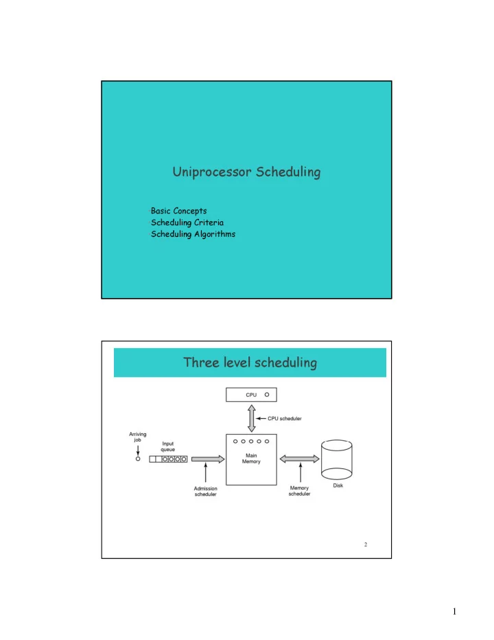
2
Uniprocessor Scheduling Basic Concepts Scheduling Criteria - - PDF document
Uniprocessor Scheduling Basic Concepts Scheduling Criteria Scheduling Algorithms Three level scheduling 2 1 Types of Scheduling 3 Long- and Medium-Term Schedulers Long-term scheduler Determines which programs are admitted to
1
2
2
3
Types of Scheduling
4
Long- and Medium-Term Schedulers
Long-term scheduler
(ie to become processes)
Medium-term scheduler
– More processes, smaller percentage of time each process is executed
3
5
Short-Term Scheduler
upon
– Clock interrupts – I/O interrupts – Operating system calls – Signals
to stop one process and start another running; the dominating factors involve:
– switching context – selecting the new process to dispatch
6
CPU–I/O Burst Cycle
cycle of
–
CPU execution and – I/O wait.
– CPU-bound – IO-bound
4
7
Scheduling Criteria- Optimization goals
CPU utilization – keep CPU as busy as possible Throughput – # of processes that complete their execution per time unit Response time – amount of time it takes from when a request was submitted until the first response is produced (execution + waiting time in ready queue)
– Turnaround time – amount of time to execute a particular process (execution + all the waiting); involves IO schedulers also
Fairness - watch priorities, avoid starvation, ... Scheduler Efficiency - overhead (e.g. context switching, computing priorities, …)
8
Nonpreemptive
terminates or blocks itself for I/O Preemptive
Ready state by the operating system
the processor for very long
5
9
First-Come-First-Served (FCFS)
wait very long before it can execute (convoy effect)
5 10 15 20 A B C E D
10
Round-Robin
5 10 15 20 A B C D E
slice or quantum -q- usually 10-100 msec)
CPU time in chunks of at most q time units
– q large ⇒ FIFO – q small ⇒ overhead can be high due to context switches
6
11
Shortest Process First
longer processes
5 10 15 20 A B C D E
12
Shortest Remaining Time First
version of shortest process next
5 10 15 20 A B C D E
7
13
On SPF Scheduling
for a given set of processes
– Proof (non-preemptive): analyze the summation giving the waiting time
– Can be done automatically (exponential averaging) – If estimated time for process (given by the user in a batch system) not correct, the operating system may abort it
14
Determining Length of Next CPU Burst
exponential averaging.
: Define 4. 1 , 3. burst CPU next the for value predicted 2. burst CPU
lenght actual 1. ≤ ≤ = =
+
α α τ
1 n th n
n t
( )
. t
n n n
τ α α τ − + =
=
1
1
8
15
On Exponential Averaging
– τn+1 = τn – history does not count, only initial estimation counts
– τn+1 = tn – Only the actual last CPU burst counts.
τn+1 = α tn+(1 - α) α tn -1 + … +(1 - α )j α tn -i + … +(1 - α )n τ0
term has less weight than its predecessor.
16
Priority Scheduling: General Rules
– can be preemptive or non-preemptive – can have multiple ready queues to represent multiple level of priority
the predicted next CPU burst time.
never execute.
priority of the process.
9
17
Priority Scheduling Cont. :
Highest Response Ratio Next (HRRN)
time spent waiting + expected service time expected service time
1 2 3 4 5 5 10 15 20
18
queues, eg
foreground (interactive) background (batch)
algorithm, eg
foreground – RR background – FCFS
queues.
– Fixed eg., serve all from foreground then from background. Possible starvation. – Another solution: Time slice – each queue gets a fraction of CPU time to divide amongst its processes, eg. 80% to foreground in RR 20% to background in FCFS
10
19
Multilevel Feedback Queue
between the various queues; aging can be implemented this way.
– number of queues – scheduling algorithm for each queue – method to upgrade a process – method to demote a process – method to determine which queue a process will enter first
20
Multilevel Feedback Queues
11
21
Fair-Share Scheduling
priority recomputation
– application runs as a collection of processes (threads) – concern: the performance of the application, user-groups, … (ie. group of processes/threads) – scheduling decisions based on process sets rather than individual processes
Real-Time Scheduling
12
23
Real-Time Systems
which occur in “real time”; process must be able to keep up, e.g.
– Control of laboratory experiments, Robotics, Air traffic control, Drive-by- wire systems, Tele/Data-communications, Military command and control systems
the computation but also on the time at which the results are produced i.e. Tasks or processes come with a deadline (for starting or completion) Requirements may be hard or soft
24
Periodic Real-TimeTasks: Timing Diagram
13
25
A movie may consist of several files
26
different for each movie (or other process that requires time guarantees)
14
27
Scheduling in Real-Time Systems Schedulable real-time system
– m periodic events – event i occurs within period Pi and requires Ci seconds
1
m i i i
=
Utilization =
28
Scheduling with deadlines: Earliest Deadline First
Set of tasks with deadlines is schedulable (i.e can be executed in a way that no process misses its deadline) iff EDF is a schedulable (aka feasible)
VI!!!
15
29
Rate Monotonic Scheduling
30
EDF or RMS? (1)
16
31
EDF or RMS? (2) Another example of real-time scheduling with RMS and EDF
32
– (recall: for EDF that is up to 1)
– main reason: stability is easier to meet with RMS; priorities are static, hence, under transient period with deadline-misses, critical tasks can be “saved” by being assigned higher (static) priorities – it is ok for combinations of hard and soft RT tasks
EDF or RMS? (3)
1
1
m i i i
C P
=
≤
0.7
17
34
18
35
36
switch
19
37
NUMA (non-uniform memory access) Multiprocessor Characteristics 1. Single address space visible to all CPUs 2. Access to remote memory via commands
3. Access to remote memory slower than to local
38
Design issues (1): Who executes the OS/scheduler(s)?
particular processor
– Master is responsible for scheduling; slave sends service request to the master – Disadvantages
– Each processor does self-scheduling – New issues for the operating system
20
39
Bus
40
Each CPU has its own operating system
Bus
21
41
– SMP multiprocessor model
Bus
42
Recall: Tightly coupled multiprocessing (SMPs)
– Processors share main memory – Controlled by operating system
Different degrees of parallelism
– Independent and Coarse-Grained Parallelism
– Medium-Grained Parallelism
– Fine-Grained Parallelism
22
43
Design issues 2: Assignment of Processes to Processors
Per-processor ready-queues vs global ready-queue
– Less overhead – A processor could be idle while another processor has a backlog
– can become a bottleneck – Task migration not cheap
44
Multiprocessor Scheduling: per partition RQ
– multiple threads at same time across multiple CPUs
23
45
Multiprocessor Scheduling: Load sharing / Global ready queue
– note use of single data structure for scheduling
46
Multiprocessor Scheduling Load Sharing: a problem
– both belong to process A – both running out of phase
24
47
Design issues 3: Multiprogramming on processors?
Experience shows: – Threads running on separate processors (to the extend of dedicating a processor to a thread) yields dramatic gains in performance – Allocating processors to threads ~ allocating pages to processes (can use working set model?) – Specific scheduling discipline is less important with more than
important
48
1. Groups of related threads scheduled as a unit (a gang) 2. All members of gang run simultaneously
3. All gang members start and end time slices together
25
49
Gang Scheduling: another option
50
Multiprocessor Thread Scheduling Dynamic Scheduling
application
parallelism
– OS adjusts the load to improve use
adjust # of threads.
26
51
Summary: Multiprocessor Thread Scheduling
Load sharing: processors/threads not assigned to particular processors
processor; cache use is less efficient
Gang scheduling: Assigns threads to particular processors (simultaneous scheduling of threads that make up a process)
application is not running (due to synchronization)
multiprogramming of processors)
52
Scheduling and synchronization
Priorities + blocking synchronization may result in: priority inversion: low-priority process P holds a lock, high- priority process waits, medium priority processes do not allow P to complete and release the lock fast (scheduling less efficient). To cope/avoid this:
– use priority inheritance – use non-blocking synchronization (wait-free, lock-free, optimistic synchronization; see some ptrs at the course’s home page)
convoy effect: processes need a resource for short time, the process holding it may block them for long time (hence, poor utilization)
– non-blocking synchronization is good here, too