Sampled data control Continuous-time system and discrete-time - - PowerPoint PPT Presentation

Sampled data control

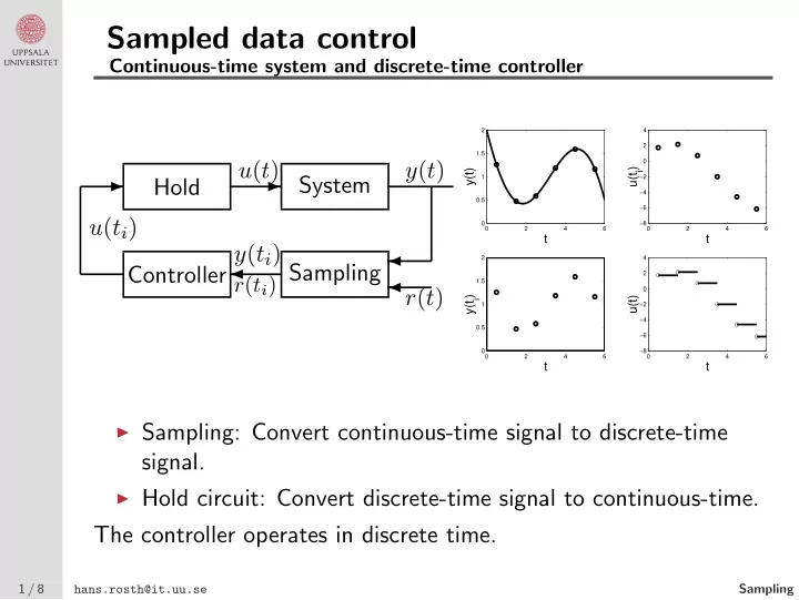
Continuous-time system and discrete-time controller

Sampling Controller Hold System

✲ ✲ ✛ ✛ ✛

r(t) y(t)

r(ti)

y(ti) u(ti) u(t)

2 4 6 0.5 1 1.5 2

y(t) t

2 4 6 −8 −6 −4 −2 2 4

u(ti) t

2 4 6 0.5 1 1.5 2

y(ti) t

2 4 6 −8 −6 −4 −2 2 4

t u(t)

◮ Sampling: Convert continuous-time signal to discrete-time

signal.

◮ Hold circuit: Convert discrete-time signal to continuous-time.

The controller operates in discrete time.

1 / 8 hans.rosth@it.uu.se Sampling

Aliasing

Can a continuous-time signal be reconstructed from discrete-time data?

Sampling period h = 1 time unit.

2 4 6 8 −1 1 time

The two sinusoids (solid and dashed lines) cannot be distinguished from each other by the sampled signal (rings).

2 / 8 hans.rosth@it.uu.se Sampling

Examples of sampled systems

The harmonic oscillator

◮ Continuous-time system:

Y (s) = 1 s2 + 1U(s) ⇔        ˙ x =

• −1

1

• x +
• 1
• u,

y =

• 1
• x

◮ Discrete-time state space model:

       x(k + 1) =

• cos(h)

− sin(h) sin(h) cos(h)

• x(k) +
• sin(h)

1 − cos(h)

• u(k),

y(k) =

• 1
• x(k).

◮ Discrete-time transfer function:

G(z) = H(zI − F)−1G = (1 − cos(h))(z + 1) z2 − 2 cos(h)z + 1

3 / 8 hans.rosth@it.uu.se Sampling

Examples of sampled systems

The double integrator

◮ Continuous-time system:

Y (s) = 1 s2 U(s) ⇔        ˙ x =

• 1
• x +
• 1
• u,

y =

• 1
• x

◮ Discrete-time state space model:

       x(k + 1) =

• 1

h 1

• x(k) +
• h

0.5h2

• u(k),

y(k) =

• 1
• x(k).

◮ Discrete-time transfer function:

G(z) =

• 1

z − 1 −h z − 1 −1 h 0.5h2

• = 0.5h2(z + 1)

(z − 1)2

4 / 8 hans.rosth@it.uu.se Sampling

Examples of sampled systems

DC motor

◮ Continuous-time system:

Y (s) = 1 s(s + 1)U(s) ⇔        ˙ x =

• −1
• x +
• 1

1

• u,

y =

• 1

−1

• x

◮ Discrete-time state space model:

       x(k + 1) =

• 1

e−h

• x(k) +
• h

1 − e−h

• u(k),

y(k) =

• 1

−1

• x(k).

◮ Discrete-time transfer function:

G(z) = H(zI − F)−1G = (h − 1 + e−h)z + 1 − (1 + h)e−h (z − 1)(z − e−h)

◮ Zero in z′ = − 1−(1+h)e−h h−1+e−h , and −1 < z′ < 0 for h > 0.

5 / 8 hans.rosth@it.uu.se Sampling

Continuous-time and sampled poles

How ZOH sampling maps the poles

• cont. time

discrete time

−1 1 −1 −0.5 0.5 1 −1 1 −1 −0.5 0.5 1 −1 1 −1 −0.5 0.5 1

6 / 8 hans.rosth@it.uu.se Sampling

Frequency response of a sampled systems

Piecewise constant sinusoids!

10 20 30 40 50 −1 −0.5 0.5 1 10 20 30 40 50 −1 −0.5 0.5 1 time

7 / 8 hans.rosth@it.uu.se Sampling

Frequency response for sampled systems

Comparison with the continuous-time frequency response

Example: Y (s) =

1 s2+s+1U(s) sampled with sampling period

h = 0.1 sec, 0.5 sec, 1 sec, 2 sec.

10

−2

10

−1

10 10

1

10

2

10

−4

10

−3

10

−2

10

−1

10 Frequency (rad/sec) Gain h = 2 sec h = 1 sec h = 0.5 sec h = 0.1 sec continuous−time system 10

−2

10

−1

10 10

1

10

2

−270 −180 −90 Frequency (rad/sec) Phase h = 2 sec h = 1 sec h = 0.5 sech = 0.1 sec Continuous−time system

Corresponding Nyquist frequencies: ωn = 31.4 rad/sec, 6.28 rad/sec, 3.14 rad/sec, 1.57 rad/s.

8 / 8 hans.rosth@it.uu.se Sampling