S.M. Iacus, D. La Torre (Univ. Milan) Different ways of simulating - PowerPoint PPT Presentation

S.M. Iacus, D. La Torre (Univ. 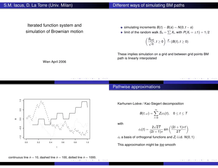Milan) Different ways of simulating BM paths Iterated function system and simulating increments B ( t ) − B ( s ) ∼ N ( 0 , t − s ) limit of the random walk S n = � X i , with P ( X i = ± 1 ) = 1 / 2 simulation of Brownian motion � S [ nt ] � d √ n , t ≥ 0 → ( B ( t ) , t ≥ 0 ) These implies simulation on a grid and between grid points BM path is linearly interpolated Wien April 2006 Pathwise approximations 1.0 Karhunen-Loève / Kac-Siegert decomposition 0.5 ∞ � B ( t , ω ) = Z i φ i ( t ) , 0 ≤ t ≤ T i = 0 0.0 B with √ 2 2 T � ( 2 i + 1 ) π t � −0.5 φ i ( t ) = ( 2 i + 1 ) π sin 2 T −1.0 φ i a basis of orthogonal functions and Z i i.i.d. N ( 0 , 1 ) 0.0 0.2 0.4 0.6 0.8 1.0 This approximation might be too smooth t continuous line n = 10, dashed line n = 100, dotted line n = 1000.

IFS-M operator The IFS-M operator is contractive operatore defined as 1.0 N � � x − a k � � � T ( g ( x )) = α k · g + β k s k 0.5 k = 1 where ( α k , β k , a k ) can be determined as the solution of a 0.0 B contrained Quadratic Problem given some choice of ( a k , s k ) ’s −0.5 ∆ 2 = || g − Tg || 2 2 = min α,β −1.0 under the constraint 0.0 0.2 0.4 0.6 0.8 1.0 N � t c k ( α k � g � 1 + β k ) ≤ � g � 1 k = 1 n = 10 (continuous line), n = 50 (dashed line) and n = 100 terms ∆ 2 can be rewritten as a quadratic form ∆ 2 = x T Ax + b T x + c 0.2 −0.2 where x = ( α 1 , . . . α k , β 1 , . . . , β k ) . If g = BM then p1 −0.6 � 1 B 2 ( t ) dt a i , i = c −1.0 0 0.0 0.2 0.4 0.6 0.8 1.0 a N + i , N + i = s i mm1 � 1 a i , N + i = c B ( t ) dt 0.4 0 � 1 0.2 b i = − 2 B ( t ) B (( t − a i ) / s i ) dt p1 0.0 0 � a i + s i −0.2 b N + i = − 2 B ( t ) dt a i 0.00 0.05 0.10 0.15 0.20 0.25 0.30 � 1 mm1 with c = 0 | B ( t ) | dt

The IFS package IFS’s can be built on distribution functions as well (DSC 2003) Theorem (Self-affine trajectories) and the ifs package include both families of operators (IFS-p Let ( α k , β k ) be the solution of ∆ 2 = min α.β then the fixed point and IFS-M) ˜ B ( t ) of the operator T satisfies the self affine property References B ( w i ( t + h )) − ˜ ˜ B ( w i ( t )) = α i (˜ B ( t + h ) − ˜ B ( t )) IFSM representation of Brownian motion with applications to simulation, submitted . where w i ( x ) = a i x + s i A comparative simulation study on the IFS distribution function estimator, Nonlinear Analysis - Real World Applications , 6 , 5, 858-873 (2005). Which means that the trajectory is made of rescaled copies of itself and here comes the fractal nature of the approximation. Approximating distribution functions by iterated function systems, Journal of Applied Mathematics and Decision Sciences , 9 , 1, 33-46 (2005).