review questions bsc3052 fst and pva 1 genetic data gives
play

Review questions BSC3052 FST and PVA 1. Genetic data gives a long - PDF document

Review questions BSC3052 FST and PVA 1. Genetic data gives a long term view on structure of populations, often we assume that the local population are in Hardy-Weinberg-equlibrium and the are able to calculate allele frequencies and using those


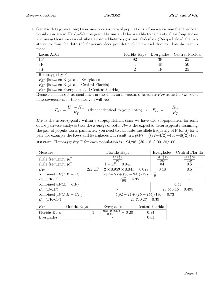
  1. Review questions BSC3052 FST and PVA 1. Genetic data gives a long term view on structure of populations, often we assume that the local population are in Hardy-Weinberg-equlibrium and the are able to calculate allele frequencies and using those we can calculate expected heterozygosities. Calculate (Recipe below) the two statistics from the data (of ’ficticious’ deer populations) below and discuss what the results mean: Locus ADH Florida Keys Everglades Central Florida FF 92 36 25 SF 4 48 50 SS 2 16 25 Homozygosity F F ST [between Keys and Everglades] F ST [between Keys and Central Florida] F ST [between Everglades and Central Florida] Recipe: calculate F as mentioned in the slides on inbreeding, calculate F ST using the expected heterozygosities, in the slides you will see F ST = H T − H W F ST = 1 − H W (this is identical to your notes) → H T H T H W is the heterozygosity within a subpopulation, since we have two subpopulation for each of the pairwise analyses take the average of both, H T is the expected heterozygosity assuming the pair of population is panmictic: you need to calculate the allele frequency of F (or S) for a pair, for example the Keys and Everglades will result in a p ( F ) = ((92+4 / 2)+(36+48 / 2) / 198. Answer: Homozygosity F for each population is : 94/98, (36+16)/100, 50/100 Measure Florida Keys Everglades Central Florida 92+ 1 36+ 1 25+ 1 2 4 2 48 2 50 allele frequency pF 98 100 100 allele frequency pS 1 − pF = 0 . 041 04 0 . 5 H W 2 pFpS = 2 × 0 . 959 × 0 . 041 = 0 . 078 0 . 48 0 . 5 ((92 + 2) + (36 + 24)) / 198 = 7 combined pF ( FK − E ) - 9 2 7 2 H T (FK-E) 9 = 0 . 35 - 9 combined pF ( E − CF ) - 0 . 55 H T (E-CF) - 20 . 550 . 45 = 0 . 495 combined pF ( FK − CF ) ((92 + 2) + (25 + 25)) / 198 = 0 . 73 H T (FK-CF) 20 . 730 . 27 = 0 . 39 F ST Florida Keys Everglades Central Florida 1 − (0 . 078+0 . 48) / 2 Florida Keys - = 0 . 20 0 . 34 0 . 35 Everglades - 0 . 01 Page: 1

  2. Review questions BSC3052 FST and PVA 2. The (ficticious) sightings of Elaphe guttata in Southwood was used to calculate transition rates from Juveniles to adults (0.255), Staying with the adult class (0.45), having 2 eggs per adult per year. http://www.uga.edu/srelherp/jd/jdweb/Herps/species/USsnakes/Elagutgut.htm • Sketch a stage graph, label all parts and fill in the transition rates. Assume that the transition rates are correct and that the snakes mature within a year. 2 Juveniles Adults 0.45 0.255 • Show the projection matrix, � � 0 2 P = 0 . 255 0 . 45 • calculate the number of juveniles and adults in year 2001 when we use the values of 2000 where we found 30 juveniles and 14 adults. Year Juveniles Adults Total 2000 30 14 44 2001 28 13.95 42 • What is the growth rate between year 2000 and 2001, compare this with the count-based method above. Growth rate λ = 42 44 [same calculaation as in count based methods once one has summed up all the stages in a year.] • Show a graph with time on the x axis and the growth rate λ on the y axis. Calculate λ for the years 2001 up to 2006 using the start condition (30 juveniles, 14 adults) Page: 2

  3. Review questions BSC3052 FST and PVA Year Juveniles Adults Total 2000 30 14 44 2001 28. 13.95 41.95 2002 27.9 13.4175 41.3175 2003 26.835 13.152375 39.9874 2004 26.30475 12.76149375 39.0662 2005 25.523 12.450 37.97 2006 24.901 12.111 37.012 [I just show the raw table of numbers a figure would include years on the X and numbers on the Y, you could plot juveniles and adults or the total. To calculate the growth rate you divide the numbers in year t by the numbers in year t-1 (for example year 2001 and 2000 λ = 41 . 95 / 44) and graph that: 0.985 0.98 0.975 0.97 0.965 4 5 2 3 6 0.955 [Y axis= growth rate, X axis = years: 1 is 2000] • How would you calculate the stable growth rate? Does your graph give a hint what the stable growth rate could be? Using the first eigenvalue of the production matrix (this is 0.973749, can be calculated in the program Populus or any other math program: matlab, maple, mathematica, I believe even in Excel). The graph is close and seems to equilibrate around that number. • Make a prognosis about the population size in year 2007 and 2008. It will continue to shrink. Page: 3

Recommend


More recommend