SLIDE 1
Review
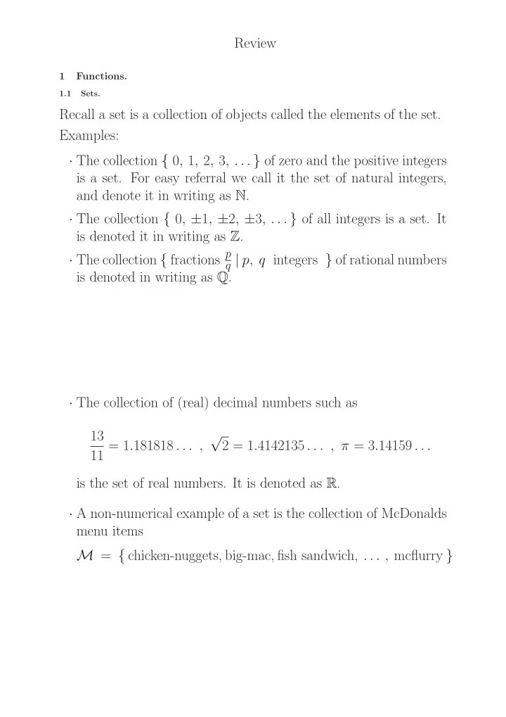
1 Functions.
1.1 Sets.
Recall a set is a collection of objects called the elements of the set. Examples: · The collection { 0, 1, 2, 3, . . . } of zero and the positive integers is a set. For easy referral we call it the set of natural integers, and denote it in writing as N. · The collection { 0, ±1, ±2, ±3, . . . } of all integers is a set. It is denoted it in writing as Z. · The collection { fractions p
q | p, q integers } of rational numbers
is denoted in writing as Q. · The collection of (real) decimal numbers such as 13 11 = 1.181818 . . . , √ 2 = 1.4142135 . . . , π = 3.14159 . . . is the set of real numbers. It is denoted as R. · A non-numerical example of a set is the collection of McDonalds menu items M = { chicken-nuggets, big-mac, fish sandwich, . . . , mcflurry }
SLIDE 2 Functions are used to express relationships among variables.
1.2 Ingredients of a function.
- Input set D
- Output set C
- Rule f
A function f is a rule which assigns to each element of the input set D, an element f(x) in the output set: x ∈ D
input
− − − − − − → rule f
− − − − − − − → f(x) ∈ C Notation:
- The input set is call the domain.
- The output set is call the codomain.
The precise set of outputs is called the range of the function.
- The output element f(x) is called the value of the function f
at input x. Example: Take · Domain (input set) to be M, the set of McDonald menu items. · Codomain (output set) to be the set N of natural integers. · function to be the price function P which is the price (in cents)
x ∈ M
input
= = = = = = = ⇒ Price function P
= = = = = = = = ⇒ P(x) ∈ N chicken-nugget
price
− − − − − − → P(chicken-nugget) So, McDonalds’ menu table is a function!
SLIDE 3 2 Ways to describe functions.
description in words
table of values
formula
by a graph Verbal example: Take: · Domain to be the alphabet A = { A, B, C, . . . , Y, Z } · Codomain to be the natural integers N. · rule p to be the position in the alphabet; so, p(B) = 2, p(L) = 12, p(Y ) = 25, etc Question: What is the range set (precise set of values) of the position function? Numerical/tabular example: Take: · Domain D to be the set URL of webnames. For example www.facebook.com ∈ D (URL). · Codomain to be the set I of all possible internet IP–addresses: aaa.bbb.ccc.ddd where each tiple is between 0 and 255 = 28 − 1 · rule f to be the ‘internet domain function’ which takes a URL x and gives the IP-number of x. For example: f(www.facebook.com) = 173.252.91.4 f(www.ust.hk) = 143.89.14.2 Each time we enter a URL into a browser, it goes to the internet to lookup the IP-address of the URL and then retrieves information stored on the machine with IP-address f(URL).
SLIDE 4 One way for hackers to disrupt the internet is by attacking the internet machines which are the repository for the function/table of URL to IP-addresses. Examples of functions given algebraically: Take: (1) f : R − → R x
f
− − − − → y = f(x) = x2 − 4 (2) g : R − → R x
g
− − − − → y = g(x) = 1 1 + x2 (3) Consider the rule: x
h
− − − − → y = h(x) = 1 x − 3 Since division by 0 is not allowed, the rule must avoid x = 3, so the domain must be the set of numbers NOT equal to 3. This set can be written in several ways such as: { x ∈ R | x = 3 }
R − { 3 }
SLIDE 5 Example of a function given graphically: Graph of the closing stock price of FaceBook during 2012-2014: Domain is the set of days. Codomain is R.
3 Vertical line test
Question: When is the set of points in the plane; for example the line x + y = 5, or the circle (x − 2)2 + (y − 2)2 = 52 the graph of a function? Vertical Line Test: A set S in the plane is the graph of a function if each vertical line meets S in at most one point. (1) The graph of the line x + y = 5 is the graph of a function. The function can be given algebraically as y = f(x) = 5 − x. (2) The graph of the circle (x − 2)2 + (y − 2)2 = 52 is not the graph
- f a function. Vertical lines x = b for −3 < b < 5 meet the circle
SLIDE 6 in two points. When we solve for y in terms of x we get (y − 2)2 = 25 − (x − 2)2 (y − 2) = ±
y = 2 ±
(3) The graph of the parabola y − x2 = 5 is the graph of a function. The function can be give algebraically as y = h(x) = 5 + x2. (4) The graph of the parabola y2 − x = 5 is the not the graph of a
- function. When we solve for y in terms of x we get
y2 = 25 − x y = ± √ 25 − x Basic Functions
4 Basic Functions.
Some basic functions given by a formula rule are:
y = f(x) = mx + b
P(x) = amxm + amxm + · · · + a2x2 + a1x + a0
r(x) = P(x) Q(x) , where P(x) and Q(x) are polynomials
Functions of the form f(x) = √x , x
1 3 ,
x−5
7 ,
. . .
sin(x), cos(x), tan(x), . . .
10x, 2x, , 3x, . . .
SLIDE 7 4.1 Linear functions.
f(x) = mx + b
- Very simple rule (easy to compute)
- Graph is a line:
· slope is m · point (0, b) is on graph, i.e., y-intercept is b
- Often used to approximate more complicated functions.
Example: CO2 levels in the atmosphere Year CO2 level (parts/million) graph point 1980 338.7 p1 = (1980, 338.7) 1988 351.5 p2 = (1988, 351.5) 1996 362.4 p3 = (1996, 362.4) 2004 377.5 p4 = (2004, 377.5) The four points do not lie on a line: The 4 input years increase by 8 years each time, but the 3 differences in the CO2 level increased by 12.8, 10.9, and 15.1 which changed from 8-year period to 8-year period to 8-year period.
SLIDE 8 Graphs of the linear function L(x) = mx + b for various slopes m and y-intercept b
330 340 350 360 370 380 390 1978 1980 1982 1984 1986 1988 1990 1992 1994 1996 1998 2000 2002 2004 2006
The best “least squares” line is the choice of slope m and y-intercept b so the function y = L(x) = m x + b has the property that for our four table values p1 = (x1, y1), p2 = (x2, y2), p3 = (x3, y3), and p4 = (x4, y4), the ‘sum of the squared differences’: ‘Error’ = ‘Error at point p1’ + ‘Error at point p2’ + ‘Error at point p3’ + ‘Error at point p4’ =
2 +
2 +
2 +
2 is the smallest possible.
SLIDE 9
Choice of slope m and intercept b Error at point p1 Error at point p2 Error at point p3 Error at point p4 Sum of errors at 4 points ( 1.6000 , -2829.3 ) (yellow) 0.00 0.00 3.61 0.16 3.77 ( 1.8875 , -3405.1 ) (green) 42.25 17.64 0.00 0.00 59.89 ( 1.6167 , -2862.3 ) (blue) 0.00 0.02 4.69 0.00 4.71 ( 1.7000 , -3015.0 ) (black) 151.29 171.61 249.64 204.49 777.03 ( 1.5912 , -2812.2 ) (red) 0.13 0.19 1.95 0.95 3.22
Calculus can be used to find the ‘best’ choice of slope m and intercept b. It is: m = 1.5912 , b = −2812.24 and y = L(x) = 1.5912 x − 2812.24 = 1.5912 ( x − 1980 ) + 338.4 . The example best least squares prediction for the CO2 levels in 2020 is L(2020) = 1.5912 ( 2020 − 1980 ) + 338.4 = 402.05 parts/million
4.2 Exponential functions.
An exponential function is defined in terms of a positive base b. For example, base 10. We know how to compute: · Integer powers of 10; 103 (thousand), 106 (million), 10−9 (nano) · Fractions powers of 10: √ 10 = 3.1622 . . . , 10
1 4 = 1.7782 . . .
It is possible to define the power 10x for any number x. For any positive base b, it is posible to define the power bx. The rule which takes input x and gives output bx is the exponential function. The function/rule is written as expb .
SLIDE 10 For example, some calculators have a button label exp10. Properties of the exponential functions are: (i) expb(1) = b (ii) expb(x + y) = expb(x) expb(y)
(turns addition into multiplication)
(iii) expb is a continuous function (iv) (bx)y = bxy Property (iii) means if we have a sequence of inputs x1, x2, x3, . . . which “converge” to a number x, then the sequence of outputs bx1, bx2, bx3, . . . converge to the output bx. This property is very
- inportant. There are ‘useless’ functions which satisfy (i) and (ii)
but not (iii).
5 One-to-one and onto functions.
Two important properties which a function may or may not have are:
and
5.1 One-to-one
A function f is one-to-one if different inputs produce different outputs We express this mathematically as saying if inputs a and b are not equal, then the outputs f(a) and f(b) are not equal. a, b ∈ D (domain), and a = b = = ⇒ f(a) = f(b) (in codomain) This is the same as: a, b ∈ D, and f(a) = f(b) = = ⇒ a = b
SLIDE 11 Examples:
L(x) = mx + b with slope m = 0 is one-to-one. Suppose x1, and x2 are two inputs which give the same output: L(x1) = L(x2). Then L(x1) = L(x2) m x1 + b = m x2 + b , so m x1 = m x2 , now divide by m = 0 x1 = x2 . Conclude a linear function L(x) = mx + b with non-zero slope is one-to-one.
- A linear function L(x) = 0 x + b with slope 0, is a constant
- function. Such functions are not one-to-one.
Horizontal line test for graph functions in the plane: If a function f is described as a graph in the plane, then f is
- ne-to-one precisely when each horizontal line in the plane meets
the graph in at most one point. If a horizontal line y = b meets the graph in two or more points p1 = (x1, b) and p2 = (x1, b), then f(x1) = f(x2) with x1 = x2, so the function is not one-to-one.
Example: sin(x) is not one-to-one, (x
3 − 1)3 + 1 is one-to-one
1 2
1 2 3 4 5
SLIDE 12 5.2 Onto
The range of a function is the complete set of its values. Examples:
- 1. The sin function has domain R. The complete set of its values
is all numbers between -1 and 1.
- 2. The function y(x) = x2 has domain R. The complete set of its
values is numbers y ≥ 0.
- 3. The function y(x) = x3 has domain R. The complete set of its
values is R For a particular function f with domain D, we usually have some choice in what we call the codomain. In each of the examples, above, we could take the codomain to be R, a larger set than the range. A function f with domain D is onto a codomain C if the codomain equals the range of the function. Examples:
- 1. Consider the sin function, with domain R.
· If we take the codomain to be R, then the sin function is not
· If we instead take the codomain to be C = { −1 ≤ y ≤ 1 }, then the function is onto the codomain.
- 2. Consider the function y(x) = x2, with domain R.
· If we take the codomain to be R, then the function is not onto the codomain. · If we instead take the codomain to be C = { 0 ≤ y }, then the function is onto the codomain.
SLIDE 13
- 3. Suppose D is a collection of at most 300 people. Take the set C
to be the the dates of the year, so C = { Jan 01, Jan 02, . . . , Dec 31 } Let B : D − − − → C, be the rule which takes input (person) x to their birthday B(x). Question: For the (365 element) codomain C, why cannot the function B be onto? A function f : D − − − → C is onto if: For any y ∈ C, there is a a ∈ D, with y = f(a) In words, any element of the codomain appears as a output/value
6 Inverse functions
When a function f : D − − − → C is both one-to-one and onto, then
- ne can “reverse” the function to get a function g : C −
− − → D. The roles of the domain and codomain have are reversed, and we think of the the process g as undoing the function f. Examples:
- 1. A linear function L(x) = mx + b from the domain R to the
codomain R, with non-zero slope m, is one-to-one and onto. The rerevse is obtained by solving for x in terms of y. It is the rule R(y) = 1 m ( y − b ) .
SLIDE 14
- 2. The rule S(x) = x2 from the domain R to the codomain R is
neither one-to-one, nor onto: · Not one-to-one since f(x) = f(−x), so different inputs can produce same output. · Not onto since the outputs (x2) are always ≥ 0, and so cannot take on any of the negative numbers in the codomain.
- 3. The same rule S(x) = x2 from the domain R≥0 to the codomain
R≥0 is both one-to-one and onto. The reverse function is the square root function: R(y) = √y , the positive square root of y.
6.1 Logarithm
When b > 1, the exponential function expb : R − − − → R>0 (note: R>0 means the positive numbers) is one-to-one and onto (the positive numbers). The inverse function is called the logarithm to base b, and denoted logb. Example:
1 2 3
1 2 3 4 5 6
f(x)= 3
x
g(x) = log (x)
3
Inverse functions
SLIDE 15
If the domain and codomain sets of a one-one and onto function f : D − − − → C are sets of real numbers, the graph of the inverse function R is obtained from the graph of f by swapping coordinates ( a , b ) ← → ( b , a ) . Geometrically the graph of the ineverse function R is obtained from the graph of f by reflection across the y = x line.
6.2 Logarithm formula between different bases
The general formula relating the functions logb and loga is: loga(x) = logb(x) logb(a) .
SLIDE 16 7 Function composition
7.1 Definition of function composition
Suppose:
- f is a function with domain D and codomain C, so
D
f
− − − − → C , and
- g is a function with domain C and codomain B, so
C
g
− − − − → B . We can form the composite function g ◦ f, which is a function with domain D and codomain B input x ∈ D
f
− − − − → f(x) ∈ C
g
− − − − →
Example: The set of real number greater than or equal to zero is denoted R≥0. Take R≥0
b(t) = √ t
− − − − − − − − − − → R≥0 (which is inside R) R≥0
c(u) =
1 1+u
− − − − − − − − − − → R≥0 The two functions b ◦ c and c ◦ b both make sense: (b ◦ c) (u) = b(c(u)) = b( 1 1 + u ) =
1 + u
is a function from R≥0 to R≥0
(c ◦ b) (t) = c(b(t)) = c( √ t ) = 1 1 + √ t
is a function from R≥0 to R≥0
SLIDE 17 7.2 Associativity of composition.
If a, b, and c are three functions, the two functions (a ◦ b) ◦ c and a ◦ (b ◦ c) are equal. Their value at an input u is: a(b(c(u))) .
8 Basic changes to the graph of a function
Suppose R
f
− − − − → R is a function with domain and range R, and a, b, c are (fixed) numbers. We can consider the functions: a f(x) , f(bx) , and f(x − c) . The relation of the graphs of these three functions to the graph of the original function f is the following:
- The graph of af(x) is obtained by vertically scaling the graph
- f f(x) by a factor of a.
- Assume b = 0. The graph of f(bx) is obtained by horizontally
scaling the graph of f(x) by a factor of 1
b.
- The graph of f(x−c) is obtained by a horizontal rightward
translation of the graph of f(x) by c.
SLIDE 18 Example: We take f(x) = x3 − 5x + 9. The graphs of (0.5)f(x) , f( x 0.8 ) , and f(x − 2) are:
5 10 15 20 25
1 2 3 4
f(x) f(x-2)