Review: integrating vector fields along curves Fix r > 0 and let - PowerPoint PPT Presentation

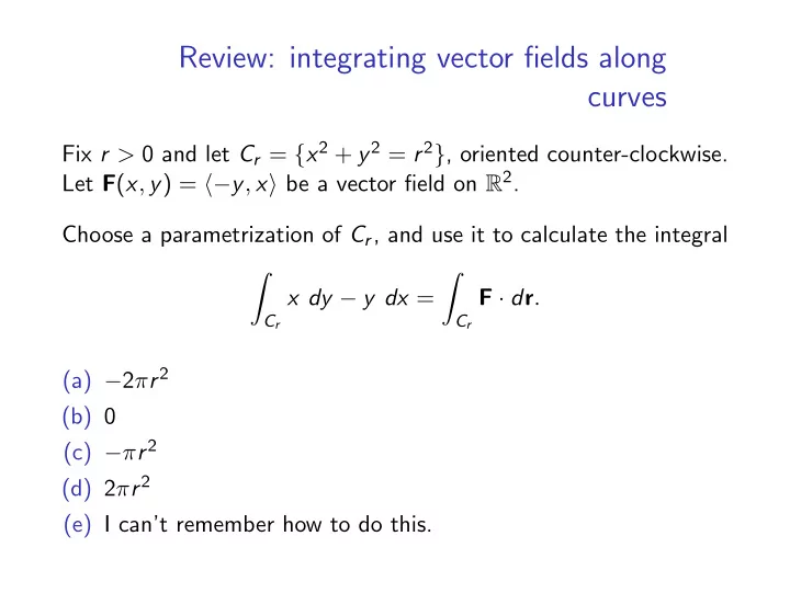
Review: integrating vector fields along curves Fix r > 0 and let C r = { x 2 + y 2 = r 2 } , oriented counter-clockwise. Let F ( x , y ) = ⟨− y , x ⟩ be a vector field on R 2 . Choose a parametrization of C r , and use it to calculate the integral ∫︂ ∫︂ x dy − y dx = F · d r . C r C r (a) − 2 π r 2 (b) 0 (c) − π r 2 (d) 2 π r 2 (e) I can’t remember how to do this.

Solution We parametrize C r by r ( t ) = ⟨ r cos t , r sin t ⟩ , 0 ≤ t ≤ 2 π, so ∫︂ 2 π ∫︂ F ( r cos t , r sin t ) · r ′ ( t ) dt x dy − y dx = C r 0 ∫︂ 2 π = ( − r sin t )( − r sin t ) + ( r cos t )( r cos t ) dt 0 ∫︂ 2 π r 2 dt = 0 = 2 π r 2 . Remember this result; we’ll need it again later.

Announcements Midterm 3 is next Tuesday, April 16, 7–8:15pm. ∙ The rooms are not the same as last time. Make sure you check the exam webpage carefully. ∙ The exam process is not quite the same as last time, either. In particular, there will be multiple versions of the exam, and the way you will be assigned seats is different. Pay attention to your TA’s instructions. ∙ If you need to take the conflict exam, you must fill out the conflict exam request form by tomorrow.

Recall some important theorems A path is a piecewise smooth curve. Fundamental Theorem of Calculus ∫︂ b f ′ ( x ) dx = f ( b ) − f ( a ) . a Fundamental Theorem of Line Integrals Let C be a path from A to B . ∫︂ ∇ f · d r = f ( B ) − f ( A ) . C Note: we have derivatives on the left, and boundary terms appearing on the right.

Assumptions for today ∙ F = ⟨ P , Q ⟩ has continuous first order partial derivatives on an open set D ⊂ R 2 . ∙ B ⊂ D is “nice”: • We can integrate over B . • The boundary ∂ B is one or more simple closed paths. ∙ We orient ∂ B so that B is always on the left.

Practice with finding area using Green’s Theorem Fix r > 0, and let B r = { x 2 + y 2 ≤ r } . Use Green’s Theorem (in particular, part (C) of the last theorem) to find the area of B r . (a) Got it! (b) I don’t see what to do yet.

Solution Note that ∂ B r = C r , the circle from the first question. So Area( B r ) = 1 ∫︂ xdy − ydx 2 C r = 1 2(2 π r 2 ) = π r 2 . (We used part (C) of the theorem, and our answer from the first question.)

Practice applying Green’s theorem − y x Let F = ⟨ x 2 + y 2 ⟩ . Recall that P y = Q x . Which of the x 2 + y 2 , following arguments is correct? (a) On C r , ⟨ P , Q ⟩ = ⟨ − y r 2 , x r 2 ⟩ , so x dy − y dx = 2 π r 2 ∫︂ F · d r = 1 ∫︂ = 2 π. r 2 r 2 C r C r (b) By Green’s Theorem, ∫︂ ∫︂∫︂ ∫︂∫︂ F · d r = ( Q x − P y ) dA = 0 dA = 0 . C r B r B r The correct answer is (a).

Using Green’s Theorem x 2 + y 2 ⟩ as before, and let C ′ be a simple closed − y x Let F = ⟨ x 2 + y 2 , curve in R 2 enclosing the origin (0 , 0). What is ∫︁ C ′ F · d r ? (a) There is not enough information to answer the question. (b) 0. (c) 2 π . (d) − 2 π . (e) I don’t know.

Solution Choose C r with r small, so that C ′ ∪ ( − C r ) is the boundary of a region B . Since F is well-behaved over B , we can use Green’s Theorem: ∫︂ ∫︂ ∫︂∫︂ C ′ F · d r + F · d r = ( Q x − P y ) dA − C r B ∫︂∫︂ = 0 dA = 0 . B So ∫︂ ′ ∫︂ 0 = F · d r − F · d r C C r And hence ∫︂ ′ ∫︂ F · d r = F · d r = 2 π. C C r