today johnson lindenstrass random subspace
play

Today Johnson-Lindenstrass Random subspace. Points: x 1 ,..., x n - PowerPoint PPT Presentation

Today Johnson-Lindenstrass Random subspace. Points: x 1 ,..., x n R d . Method 1: Random k = c log n dimensional subspace. Pick unit v 1 , 2 v 2 orthogonal to v 1 , 1 Claim: with probability 1 n c 2 , ... v k orthogonal to


  1. Today Johnson-Lindenstrass Random subspace. Points: x 1 ,..., x n ∈ R d . Method 1: Random k = c log n dimensional subspace. Pick unit v 1 , ε 2 v 2 orthogonal to v 1 , 1 Claim: with probability 1 − n c − 2 , ... v k orthogonal to previous vectors... � � k k d | x i − x j | 2 ≤ | y i − y j | 2 ≤ ( 1 + ε ) d | x i − x j | 2 ( 1 − ε ) Method 2: Choose k vectors v 1 ,..., v k Gram Schmidt orthonormalization of k × d matrix where rows are v i . � d “Projecting and scaling by k preserves all pairwise distances w/in remove projection onto previous subspace. factor of 1 ± ε .” Projections. Expected value of y i . 
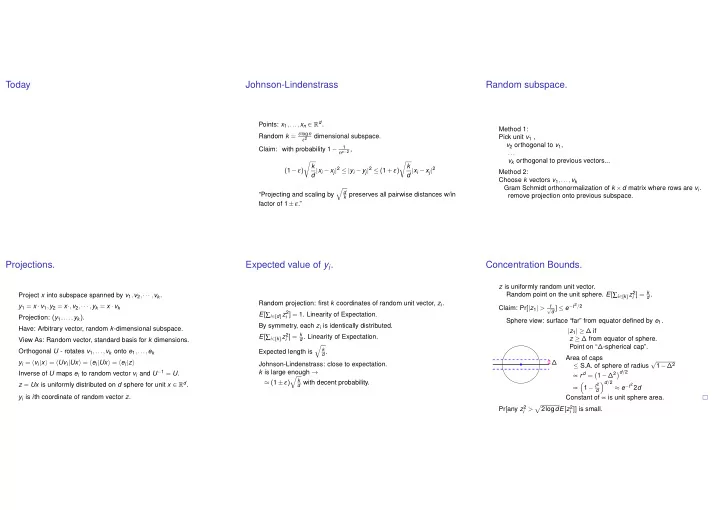
Concentration Bounds. z is uniformly random unit vector. Random point on the unit sphere. E [ ∑ i ∈ [ k ] z 2 i ] = k Project x into subspace spanned by v 1 , v 2 , ··· , v k . d . Random projection: first k coordinates of random unit vector, z i . y 1 = x · v 1 , y 2 = x · , v 2 , ··· , y k = x · v k d ] ≤ e − t 2 / 2 t Claim: Pr [ | z 1 | > √ E [ ∑ i ∈ [ d ] z 2 i ] = 1. Linearity of Expectation. Projection: ( y 1 ,..., y k ) . Sphere view: surface “far” from equator defined by e 1 . By symmetry, each z i is identically distributed. Have: Arbitrary vector, random k -dimensional subspace. | z 1 | ≥ ∆ if i ] = k E [ ∑ i ∈ [ k ] z 2 d . Linearity of Expectation. z ≥ ∆ from equator of sphere. View As: Random vector, standard basis for k dimensions. Point on “ ∆ -spherical cap”. � k Orthogonal U - rotates v 1 ,..., v k onto e 1 ,..., e k Expected length is d . Area of caps √ y i = � v i | x � = � Uv i | Ux � = � e i | Ux � = � e i | z � ∆ Johnson-Lindenstrass: close to expectation. 1 − ∆ 2 ≤ S.A. of sphere of radius Inverse of U maps e i to random vector v i and U − 1 = U . k is large enough → ∝ r d = 1 − ∆ 2 � d / 2 � � k ≈ ( 1 ± ε ) d with decent probability. � d / 2 z = Ux is uniformly distributed on d sphere for unit x ∈ R d . � 1 − t 2 ≈ e − t 2 2 d ∝ d y i is i th coordinate of random vector z . Constant of ∝ is unit sphere area. Pr [ any z 2 � 2log dE [ z 2 i > i ]] is small.

  2. Many coordinates. Locality Preserving Hashing Implementing Johnson-Lindenstraus Proved Pr [ any z 2 � 2log dE [ z 2 i > i ]] is small. Length? z = z 2 1 + z 2 2 + ··· z 2 k . � � � � � > t ] ≤ e − t 2 d � z 2 1 + z 2 2 + ··· + z 2 k � Pr [ k − Find nearby points in high dimensional space. Random vectors have many bits � � d � Points could be images! Use random bit vectors: {− 1 , + 1 } d instead. � d , k = c log n k Substituting t = ε ε 2 . Hash function h ( · ) s.t. h ( x i ) = h ( x j ) if d ( x i , x j ) ≤ δ . Almost orthogonal. √ � � Low dimensions: grid cells give d -approximation. � � � d ] ≤ e − ε 2 k = e − c log n = 1 � z 2 1 + z 2 2 + ··· + z 2 k � k Pr [ k − � > ε Project z . � � n c Not quite a solution. Why? d � Close to grid boundary. Coordinate for bit vector b . Johnson-Lindenstraus: For n points, x 1 ,..., x n , all distances 1 Find close points to x : C i = √ d ∑ i b i z i � k preserved to within 1 ± ε under d -scaled projection above. Check grid cell and neighboring grid cells. E [ C 2 i ] = E [ 1 d ∑ i , j b i b j z i z j ] = 1 d ∑ i , j E [ b i b j ] z i z j = 1 d ∑ i z 2 i = 1 d View one pair x i − x j as vector. Project high dimensional points into low dimensions. E [ ∑ i C 2 i ] = k Scale to unit. d Use grid hash function. Projection fails to preserve | x i − x j | with probability ≤ 1 n c Scaled vector length also preserved. ≤ n 2 pairs plus union bound 1 → prob any pair fails to be preserved with ≤ n c − 2 . Binary Johnson-Lindenstrass Analysis Idea. Sum up � | C − k d | ≥ ε k � ≤ e − ε 2 k Pr Project onto [ − 1 , + 1 ] vectors. d E [ C ] = E [ ∑ i C 2 i ] = k � � � � d ( ∑ i z i 4 + 4 ∑ i , j z 2 i ) 2 ≤ 2 k Variance of C 2 k i z 2 k 2 ( ∑ i z 2 j ) ≤ i ? d 2 . d 2 d 2 Concentration? Roughly normal (gaussian): Density ∝ e − t 2 / 2 for t std deviations away. � | C − k d | ≥ ε k � ≤ e − ε 2 k Pr d So, assuming normality √ √ √ ε k k σ = d , t = d = ε k / 2 . √ Choose k = c log n ε 2 . 2 k d → failure probability ≤ 1 / n c . Probability of failure roughly ≤ e − t 2 / 2 → e ε 2 k / 4 “Roughly normal.” Chernoff, Berry-Esseen, Central Limit Theorems.

  3. Have a good break!

Download Presentation
Download Policy: The content available on the website is offered to you 'AS IS' for your personal information and use only. It cannot be commercialized, licensed, or distributed on other websites without prior consent from the author. To download a presentation, simply click this link. If you encounter any difficulties during the download process, it's possible that the publisher has removed the file from their server.

Recommend


More recommend