Regular Markov Chains MATH 107: Finite Mathematics University of - PDF document

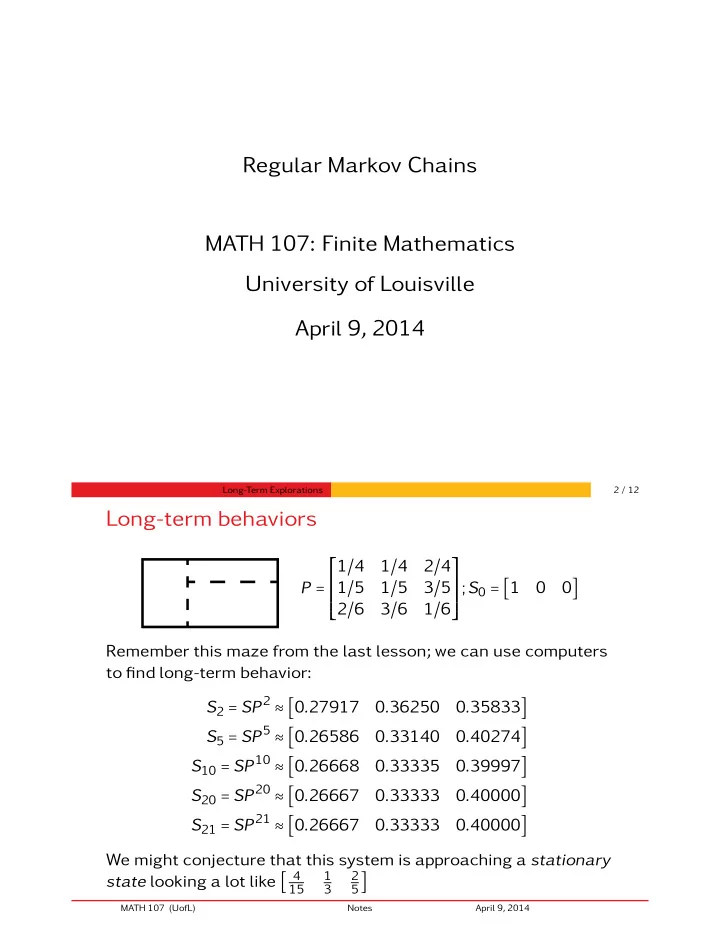
Regular Markov Chains MATH 107: Finite Mathematics University of Louisville April 9, 2014 Long-Term Explorations 2 / 12 Long-term behaviors ⎡ ⎤ 1 / 4 1 / 4 2 / 4 ⎢ ⎥ ⎢ ⎥ P = ⎢ 1 / 5 1 / 5 3 / 5 ⎥ ; S 0 = [ 1 0 ] ⎢ ⎥ 0 ⎢ ⎥ 2 / 6 3 / 6 1 / 6 ⎣ ⎦ Remember this maze from the last lesson; we can use computers to find long-term behavior: S 2 = SP 2 ≈ [ 0 . 27917 0 . 35833 ] 0 . 36250 S 5 = SP 5 ≈ [ 0 . 26586 0 . 40274 ] 0 . 33140 S 10 = SP 10 ≈ [ 0 . 26668 0 . 39997 ] 0 . 33335 S 20 = SP 20 ≈ [ 0 . 26667 0 . 40000 ] 0 . 33333 S 21 = SP 21 ≈ [ 0 . 26667 0 . 40000 ] 0 . 33333 We might conjecture that this system is approaching a stationary state looking a lot like [ 4 5 ] 1 2 15 3 MATH 107 (UofL) Notes April 9, 2014

Long-Term Explorations 3 / 12 More long-term behavior ⎡ ⎤ ⎢ ⎥ ⎢ ⎥ 0 1 0 ⎢ ⎥ ; S 0 = [ 0 . 2 0 . 5 ] ⎢ ⎥ 0 . 3 0 . 0 0 . 7 0 . 3 ⎢ ⎥ ⎣ ⎦ 0 1 0 Alas, not every transition matrix reaches a stationary state! S 1 = SP = [ 0 . 09 0 . 21 ] 0 . 70 S 2 = SP 2 = [ 0 . 21 0 . 49 ] 0 . 30 S 3 = SP 3 = [ 0 . 09 0 . 21 ] 0 . 70 and the system oscillates between these two states forever! Key questions ▸ When does a system have a unique stationary state? ▸ What is that stationary state? MATH 107 (UofL) Notes April 9, 2014 Regular Markov Chains 4 / 12 Stationary states ⎡ ⎤ ⎢ ⎥ ⎢ ⎥ 0 1 0 ⎢ ⎥ ⎢ ⎥ Some matrices, like 0 . 3 0 . 0 0 . 7 , have no stationary state. ⎢ ⎥ ⎣ ⎦ 0 1 0 ⎡ ⎤ ⎢ ⎥ ⎢ ⎥ 1 0 0 ⎢ ⎥ ⎢ ⎥ 0 0 . 5 0 . 5 Some, like have many stationary states. ⎢ ⎥ ⎣ ⎦ 0 0 . 3 0 . 7 We want to know which transition matrices have exactly one stationary state. MATH 107 (UofL) Notes April 9, 2014

Regular Markov Chains 5 / 12 The regularity criterion Definition A matrix P is regular if there is some number n such that every entry of P n is nonzero. A Markov chain is regular if its transition matrix is regular. ⎡ ⎤ 1 / 4 1 / 4 2 / 4 ⎢ ⎥ ⎢ ⎥ ⎢ 1 / 5 1 / 5 3 / 5 ⎥ ⎢ ⎥ So, for instance, our maze example is regular, ⎢ ⎥ 2 / 6 3 / 6 1 / 6 ⎣ ⎦ ⎡ ⎤ ⎡ ⎤ ⎢ ⎥ ⎢ ⎥ ⎢ ⎥ ⎢ ⎥ 0 1 0 1 0 0 ⎢ ⎥ ⎢ ⎥ ⎢ ⎥ ⎢ ⎥ and the matrices 0 . 3 0 . 0 0 . 7 and 0 0 . 5 0 . 5 are not. ⎢ ⎥ ⎢ ⎥ ⎣ ⎦ ⎣ ⎦ 0 1 0 0 0 . 3 0 . 7 Theorem A Markov chain has a unique stationary state if and only if it is regular. We won’t prove that here; details are in MATH 325. MATH 107 (UofL) Notes April 9, 2014 Regular Markov Chains 6 / 12 Testing regularity To determine whether a matrix is regular, we look at powers of it until either we have all nonzero entries or we repeat entries. Fortunately, in doing this test, we only need consider whether entries are zero or nonzero, not their arithmetic values. Example ⎡ ⎤ ⎢ ⎥ ⎢ ⎥ 0 0 . 3 0 . 7 Is P = ⎢ ⎥ ⎢ ⎥ 0 . 5 0 0 . 5 regular? ⎢ ⎥ ⎣ ⎦ 1 0 0 ⎡ ⎤ ⎡ ⎤ ⎡ ⎤ ⎡ ⎤ ∼ ∼ ∼ ∼ ∼ ∼ ∼ ∼ ∼ ∼ ⎢ ⎥ ⎢ ⎥ ⎢ ⎥ ⎢ ⎥ ⎢ ⎥ ⎢ ⎥ ⎢ ⎥ ⎢ ⎥ 0 0 ; P 2 = ; P 3 = ; P 4 = P = ⎢ ∼ ∼ ⎥ ⎢ ∼ ∼ ∼ ⎥ ⎢ ∼ ∼ ∼ ⎥ ⎢ ∼ ∼ ∼ ⎥ ⎢ ⎥ ⎢ ⎥ ⎢ ⎥ ⎢ ⎥ 0 ⎢ ⎥ ⎢ ⎥ ⎢ ⎥ ⎢ ⎥ ∼ ∼ ∼ ∼ ∼ ∼ ∼ ∼ ⎣ ⎦ ⎣ ⎦ ⎣ ⎦ ⎣ ⎦ 0 0 0 0 , so P is regular! MATH 107 (UofL) Notes April 9, 2014

Stationary states 7 / 12 Finding stationary vectors Having determined when a matrix has a stationary state, we now want to find that state. What we want is a vector S such that SP = S . Also, since S describes a probability or proportion, we need its entries to add up to 1. SP = S ⇒ SP = SI n ⇒ SP − SI n = 0 ⇒ S ( P − I n ) = 0 and in addition the entries of S add up to 1. If we name the entries of S , we can thus solve the associated system. MATH 107 (UofL) Notes April 9, 2014 Stationary states 8 / 12 Case study: mouse in a maze ⎡ ⎤ 1 / 4 1 / 4 2 / 4 ⎢ ⎥ ⎢ ⎥ P = ⎢ 1 / 5 1 / 5 3 / 5 ⎥ ⎢ ⎥ ⎢ ⎥ 2 / 6 3 / 6 1 / 6 ⎣ ⎦ This is our “mouse-in-a-maze” transition matrix. Let’s find a stationary S = [ s 1 s 3 ] . s 2 S ( P − I 3 ) = 0 and s 1 + s 2 + s 3 = 1 ⎧ − 3 4 s 1 + 1 5 s 2 + 1 3 s 3 = 0 ⎪ ⎡ ⎤ ⎪ − 3 / 4 1 / 4 1 / 2 ⎪ ⎢ ⎥ ⎪ ⎪ ⎢ ⎥ ⎪ ⎪ 4 s 1 − 4 5 s 2 + 1 2 s 3 = 0 [ s 1 s 3 ] ⎢ 1 / 5 − 4 / 5 3 / 5 ⎥ = [ 0 0 ] ⎪ 1 ⎢ ⎥ ⇒ ⎨ 0 s 2 ⎢ ⎥ 1 / 3 1 / 2 − 5 / 6 ⎪ 2 s 1 + 3 5 s 2 − 5 6 s 3 = 0 ⎪ ⎣ ⎦ ⎪ ⎪ 1 ⎪ s 1 + s 2 + s 3 = 1 ⎪ ⎪ ⎪ s 1 + s 2 + s 3 = 1 ⎩ MATH 107 (UofL) Notes April 9, 2014

Stationary states 9 / 12 Case study: mouse in a maze (cont’d) ⎧ − 3 4 s 1 + 1 5 s 2 + 1 3 s 3 = 0 ⎧ ⎪ 45 s 1 − 12 s 2 − 20 s 3 = 0 ⎪ ⎪ ⎪ ⎪ ⎪ ⎪ ⎪ ⎪ ⎪ ⎪ ⎪ ⎪ 4 s 1 − 4 5 s 2 + 1 2 s 3 = 0 5 s 1 − 16 s 2 + 10 s 3 = 0 ⎪ ⎪ 1 ⎨ � ⇒ ⎨ ⎪ ⎪ 15 s 1 + 18 s 2 − 25 s 3 = 0 ⎪ 2 s 1 + 3 5 s 2 − 5 6 s 3 = 0 ⎪ ⎪ ⎪ ⎪ ⎪ 1 ⎪ ⎪ ⎪ ⎪ ⎪ ⎪ s 1 + s 2 + s 3 = 1 ⎪ s 1 + s 2 + s 3 = 1 ⎩ ⎩ ⎡ ⎤ − 12 − 20 ⎢ ⎥ ⎢ 45 0 ⎥ − 16 ⎢ ⎥ ⎢ ⎥ 5 10 0 ⎢ ⎥ − 25 which we can solve by reducing . ⎢ ⎥ 15 18 0 ⎢ ⎥ ⎣ ⎦ 1 1 1 1 ⎡ ⎤ ⎡ ⎤ − 12 − 20 ⎢ ⎥ ⎢ ⎥ 4 1 0 0 ⎢ 45 0 ⎥ ⎢ ⎥ − 16 15 ⎢ ⎥ ⎢ ⎥ 1 ⎢ ⎥ ∼ ⎢ ⎥ 5 10 0 0 1 0 ⎢ ⎥ ⎢ ⎥ − 25 3 ⎢ ⎥ ⎢ ⎥ 2 15 18 0 0 0 1 ⎢ ⎥ ⎢ ⎥ 5 ⎣ ⎦ ⎣ ⎦ 1 1 1 1 0 0 0 0 which is the result we expected way back when! MATH 107 (UofL) Notes April 9, 2014 Stationary states 10 / 12 Case study: ine ff ective vaccine ⎡ ⎤ ⎢ ⎥ ⎢ ⎥ 0 . 95 0 0 . 05 P = ⎢ ⎥ ⎢ ⎥ 0 . 3 0 . 5 0 . 2 ⎢ ⎥ ⎣ ⎦ 0 0 . 5 0 . 5 This is our vaccination transition matrix from the last lecture. Let’s find a stationary S = [ s 1 s 3 ] . s 2 ⎡ ⎤ − 0 . 05 ⎢ ⎥ ⎢ ⎥ 0 0 . 05 [ s 1 s 3 ] ⎢ − 0 . 5 ⎥ = [ 0 0 ] ⎢ ⎥ s 2 0 . 3 0 . 2 0 ⎢ ⎥ − 0 . 5 ⎣ ⎦ 0 0 . 5 s 1 + s 2 + s 3 = 1 ⎧ − 0 . 05 s 1 + 0 . 3 s 2 = 0 ⎪ ⎪ ⎪ ⎪ ⎪ ⎪ s 1 − 0 . 5 s 2 + 0 . 5 s 3 = 0 ⎪ ⎨ 0 ⎪ 0 . 05 s 1 + 0 . 2 s 2 − 0 . 5 s 3 = 0 ⎪ ⎪ ⎪ ⎪ ⎪ ⎪ s 1 + s 2 + s 3 = 1 ⎩ MATH 107 (UofL) Notes April 9, 2014

Stationary states 11 / 12 Case study: ine ff ective vaccine (cont’d) ⎧ ⎧ − 0 . 05 s 1 + 0 . 3 s 2 = 0 5 s 1 − 30 s 2 = 0 ⎪ ⎪ ⎪ ⎪ ⎪ ⎪ ⎪ ⎪ ⎪ ⎪ ⎪ ⎪ − 0 . 5 s 2 + 0 . 5 s 3 = 0 s 2 − s 3 = 0 ⎪ ⎪ ⎨ � ⇒ ⎨ ⎪ ⎪ 0 . 05 s 1 + 0 . 2 s 2 − 0 . 5 s 3 = 0 5 s 1 + 20 s 2 − 50 s 3 = 0 ⎪ ⎪ ⎪ ⎪ ⎪ ⎪ ⎪ ⎪ ⎪ ⎪ ⎪ ⎪ s 1 + s 2 + s 3 = 1 s 1 + s 2 + s 3 = 1 ⎩ ⎩ ⎡ ⎤ − 30 ⎢ ⎥ ⎢ 5 0 0 ⎥ − 1 ⎢ ⎥ ⎢ ⎥ 0 1 0 ⎢ ⎥ − 50 which we can solve by reducing . ⎢ ⎥ 5 20 0 ⎢ ⎥ ⎣ ⎦ 1 1 1 1 ⎡ ⎤ ⎡ ⎤ − 30 ⎢ ⎥ ⎢ ⎥ 3 5 0 0 1 0 0 ⎢ ⎥ ⎢ ⎥ − 1 ⎢ ⎥ ⎢ 4 ⎥ ⎢ ⎥ ∼ ⎢ 1 ⎥ 0 1 0 0 1 0 ⎢ ⎥ ⎢ ⎥ − 50 8 ⎢ ⎥ ⎢ ⎥ 1 5 20 0 0 0 1 ⎢ ⎥ ⎢ ⎥ 8 ⎣ ⎦ ⎣ ⎦ 1 1 1 1 0 0 0 0 so 75% of the population will end up vaccinated long-term, while the remaining 25% are evenly split between being well and ill. MATH 107 (UofL) Notes April 9, 2014 Stationary states 12 / 12 A more typical example: 2-state systems Mercifully, you will usually be spared 3-state systems. More usually you will be given a 2-state system. Commuter preferences Every month, 20% of rapid transit users switch to driving, while 30% of car drivers switch to rapid transit. What is the long-term proportion of drivers to transit users? 0 . 7 ]← RT Here, P = [ 0 . 8 0 . 2 ← Car . 0 . 3 s 2 ][ − 0 . 2 And we want a solution to [ s 1 − 0 . 3 ] = [ 0 0 ] 0 . 2 0 . 3 with s 1 + s 2 = 1. Thus, we have the system ⎧ − 0 . 2 s 1 + 0 . 3 s 2 = 0 ⎪ ⎪ ⎪ ⎪ ⎨ 0 . 2 s 1 − 0 . 3 s 2 = 0 ⎪ ⎪ ⎪ ⎪ s 1 + s 2 = 1 ⎩ MATH 107 (UofL) Notes April 9, 2014

Stationary states 13 / 12 2-state systems (cont’d) ⎧ − 0 . 2 s 1 + 0 . 3 s 2 = 0 ⎪ ⎪ ⎪ ⇒ { 2 s 1 − 3 s 2 = 0 ⎪ ⎨ 0 . 2 s 1 − 0 . 3 s 2 = 0 ⎪ s 1 + s 2 = 1 ⎪ ⎪ ⎪ s 1 + s 2 = 1 ⎩ We could use, for instance, substitution to solve this: s 1 = 3 2 s 2 , so: 2 s 2 + s 2 = 1 ⇒ 5 2 s 2 = 1 ⇒ s 2 = 2 3 5 and then s 1 = 3 2 × 2 5 = 3 5 . Thus 60% of the population would use rapid transit and 40% cars. MATH 107 (UofL) Notes April 9, 2014