Recap: Q-Learning with state abstraction Using a feature - - PowerPoint PPT Presentation

Recap: Q-Learning with state abstraction

1

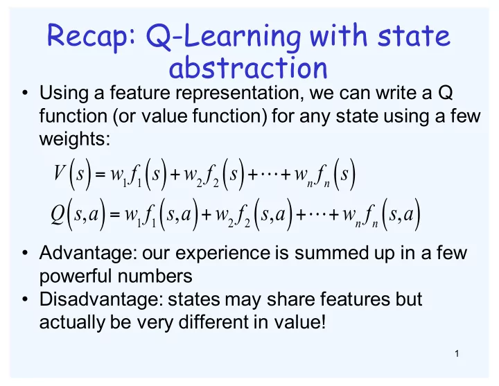
• Using a feature representation, we can write a Q

function (or value function) for any state using a few weights:

• Advantage: our experience is summed up in a few

powerful numbers

• Disadvantage: states may share features but

actually be very different in value!

V s

( ) = w1 f1 s ( )+ w2 f2 s ( )++ wn fn s ( )

Q s,a

( ) = w1 f1 s,a ( )+ w2 f2 s,a ( )++ wn fn s,a ( )

Function Approximation

2

• Q-learning with linear Q-functions:

transition = (s,a,r,s’)

• Intuitive interpretation:

– Adjust weights of active features – E.g. if something unexpectedly bad happens, disprefer all states with that state’s features

• Formal justification: online least squares

Q s,a

( ) = w1 f1 s,a ( )+ w2 f2 s,a ( )++ wn fn s,a ( )

( )

'

difference max ', ' ( , )

a

r Q s a Q s a γ ⎡ ⎤ = + − ⎣ ⎦

Q(s,a) ← Q(s,a)+α difference " # $ % wi ← wi +α difference " # $ % fi s,a

( )

Exact Q’s Approximate Q’s

Example: Q-Pacman

3

Q(s,a)= 4.0fDOT(s,a)-1.0fGST(s,a) fDOT(s,NORTH)=0.5 fGST(s,NORTH)=1.0 Q(s,a)=+1 R(s,a,s’)=-500 difference=-501 wDOT←4.0+α[-501]0.5 wGST ←-1.0+α[-501]1.0 Q(s,a)= 3.0fDOT(s,a)-3.0fGST(s,a)

α= North r = -500 s s’

Today: Reasoning over Time

4

• Often, we want to reason about a sequence of
• bservations

– Speech recognition – Robot localization – User attention – Medical monitoring

• Need to introduce time into our models
• Basic approach: hidden Markov models (HMMs)
• More general: dynamic Bayes’ nets

Markov Models

5

• A Markov model is a chain-structured BN

– Conditional probabilities are the same (stationarity) – Value of X at a given time is called the state – As a BN: – Parameters: called transition probabilities or dynamics, specify how the state evolves over time (also, initial probabilities)

p(X1) p(X|X-1)

Example: Markov Chain

6

• Weather:

– States: X = {rain, sun} – Transitions: – Initial distribution: 1.0 sun – What’s the probability distribution after one step?

p(X2=sun)=p(X2=sun|X1=sun)p(X1=sun)+ p(X2=sun|X1=rain)p(X1=rain) =0.9*1.0+1.0*0.0 =0.9

Forward Algorithm

7

• Question: What’s p(X) on some day t?

( ) ( ) ( ) ( )

1

1 1 1

| known

t

t t x t t

p x p x p x p x x

−

− −

= =

∑

Forward simulation

Example

8

• From initial observation of sun
• From initial observation of rain

p(X1) p(X2) p(X3) p(X∞) p(X1) p(X2) p(X3) p(X∞)

Stationary Distributions

9

• If we simulate the chain long enough:

– What happens? – Uncertainty accumulates – Eventually, we have no idea what the state is!

• Stationary distributions:

– For most chains, the distribution we end up in is independent of the initial distribution – Called the stationary distribution of the chain – Usually, can only predict a short time out

• p(X=sun)=p(X=sun|X-1=sun)p(X=sun)+

p(X=sun|X-1=rain)p(X=rain)

• p(X=rain)=p(X=rain|X-1=sun)p(X=sun)+

p(X=rain|X-1=rain)p(X=rain)

10

Computing the stationary distribution

Web Link Analysis

11

• PageRank over a web graph

– Each web page is a state – Initial distribution: uniform over pages – Transitions:

• With prob. c, uniform jump to a random

page (dotted lines, not all shown)

• With prob. 1-c, follow a random outlink (solid lines)
• Stationary distribution

– Will spend more time on highly reachable pages – Somewhat robust to link spam

Restrictiveness of Markov models

• Are past and future really independent given current state?
• E.g., suppose that when it rains, it rains for at most 2 days

X1 X2 X3 X4 …

• Second-order Markov process
• Workaround: change meaning of “state” to events of last 2 days

X1, X2

…

X2, X3 X3, X4 X4, X5

• Another approach: add more information to the state
• E.g., the full state of the world would include whether the

sky is full of water

– Additional information may not be observable – Blowup of number of states…

Hidden Markov Models

13

• Markov chains not so useful for most agents

– Eventually you don’t know anything anymore – Need observations to update your beliefs

• Hidden Markov models (HMMs)

– Underlying Markov chain over state X – You observe outputs (effects) at each time step – As a Bayes’ net:

Example

14

• An HMM is defined by:

– Initial distribution: p(X1) – Transitions: p(X|X-1) – Emissions: p(E|X)

Rt-1 p(Rt) t 0.7 f 0.3 Rt p(Ut) t 0.9 f 0.2

Conditional Independence

15

• HMMs have two important independence properties:

– Markov hidden process, future depends on past via the present – Current observation independent of all else given current state

• Quiz: does this mean that observations are

independent?

– [No, correlated by the hidden state]

Real HMM Examples

16

• Speech recognition HMMs:

– Observations are acoustic signals (continuous values) – States are specific positions in specific words (so, tens of thousands)

• Robot tracking:

– Observations are range readings (continuous) – States are positions on a map (continuous)

Filtering / Monitoring

17

• Filtering, or monitoring, is the task of tracking the

distribution B(X) (the belief state) over time

• We start with B(X) in an initial setting, usually

uniform

• As time passes, or we get observations, we update

B(X)

• The Kalman filter was invented in the 60’s and first

implemented as a method of trajectory estimation for the Apollo program

Example: Robot Localization

18

May not execute action with small prob.

Example: Robot Localization

19

Example: Robot Localization

20

Example: Robot Localization

21

Example: Robot Localization

22

Example: Robot Localization

23

Another weather example

• Xt is one of {s, c, r} (sun, cloudy, rain)
• Transition probabilities:

s c r

.1 .2 .6 .3 .4 .3 .3 .5 .3 not a Bayes net!

• Throughout, assume uniform distribution over X1

Weather example extended to HMM

• Transition probabilities:

s c r

.1 .2 .6 .3 .4 .3 .3 .5 .3

• Observation: roommate wet or dry
• p(w|s) = .1, p(w|c) = .3, p(w|r) = .8

HMM weather example: a question

s c r

.1 .2 .6 .3 .4 .3 .3 .5 .3

• You have been stuck in the dorm for three days (!)
• On those days, your roommate was dry, wet, wet,

respectively

• What is the probability that it is now raining outside?
• p(X3 = r | E1 = d, E2 = w, E3 = w)
• By Bayes’ rule, really want to know p(X3, E1 = d, E2 = w, E3 = w)

p(w|s) = .1 p(w|c) = .3 p(w|r) = .8

Solving the question

• Computationally efficient approach: first compute

p(X1 = i, E1 = d) for all states i

• General case: solve for p(Xt, E1 = e1, …, Et = et) for

t=1, then t=2, … This is called monitoring

• p(Xt, E1 = e1, …,Et = et) = ΣXt-1 p(Xt-1 = xt-1, E1 = e1, …,

Et-1 = et-1) P(Xt| Xt-1 = xt-1) P(Et = et | Xt)

s c r

.1 .2 .6 .3 .4 .3 .3 .5 .3

p(w|s) = .1 p(w|c) = .3 p(w|r) = .8

Predicting further out

• You have been stuck in the dorm for three days
• On those days, your roommate was dry, wet, wet,

respectively

• What is the probability that two days from now it

will be raining outside?

• p(X5 = r | E1 = d, E2 = w, E3 = w)

s c r

.1 .2 .6 .3 .4 .3 .3 .5 .3

p(w|s) = .1 p(w|c) = .3 p(w|r) = .8

Predicting further out, continued…

• Want to know: p(X5 = r | E1 = d, E2 = w, E3 = w)
• Already know how to get: p(X3 | E1 = d, E2 = w, E3 = w)
• p(X4 = r | E1 = d, E2 = w, E3 = w) =

ΣX3 P(X4 = r, X3 = x3 | E1 = d, E2 = w, E3 = w) =ΣX3 P(X4 = r | X3 = x3)P(X3 = x3 | E1 = d, E2 = w, E3 = w)

• Etc. for X5
• So: monitoring first, then straightforward Markov process

updates

s c r

.1 .2 .6 .3 .4 .3 .3 .5 .3

p(w|s) = .1 p(w|c) = .3 p(w|r) = .8

Integrating newer information

s c r

.1 .2 .6 .3 .4 .3 .3 .5 .3

• You have been stuck in the dorm for four days (!)
• On those days, your roommate was dry, wet, wet, dry

respectively

• What is the probability that two days ago it was raining
• utside? p(X2 = r | E1 = d, E2 = w, E3 = w, E4 = d)

– Smoothing or hindsight problem

p(w|s) = .1 p(w|c) = .3 p(w|r) = .8