Regression Models Bivariate data (y,x) Multivariate (y,x 1 ,,x k ) - - PowerPoint PPT Presentation

Regression Models

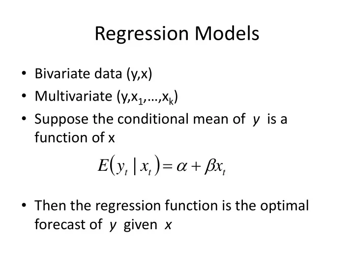
• Bivariate data (y,x)
• Multivariate (y,x1,…,xk)
• Suppose the conditional mean of y is a

function of x

• Then the regression function is the optimal

forecast of y given x

( )

t t t

x x y E β α + = |

Regression

• Model
• Estimation: Least-Squares
• Example: Interest Rates

– Monthly – Rates on 3-month and 1-year U.S. Treasury Bonds – 3-month bond series dates from 1934m1 – 1-year bond series dates from 1953m4

t t t

e x y + + = β α

Interest Rates on Treasury Bonds

5 10 15 20 1940m1 1960m1 1980m1 2000m1 2020m1 time 3-Month Treasury One-Year Treasury

Least-Squares, 3-month on 1-year rate

t t

x y 93 . 18 . ˆ + − =

_cons -.1826507 .0261585 -6.98 0.000 -.2340043 -.1312971 t1year .9344078 .0064224 145.49 0.000 .9217994 .9470161 t3month Coef. Std. Err. t P>|t| [95% Conf. Interval] Robust Root MSE = .35034 R-squared = 0.9869 Prob > F = 0.0000 F( 1, 741) =21167.67 Linear regression Number of obs = 743 . reg t3month t1year, r

Forecast

• A forecast of yn+h requires xn+h
• This is not typically feasible, as xn+h is

unknown at time n.

h n h n h n

e x y

+ + +

+ + = β α

h n n h n

x y

+ +

+ = β α

|

ˆ

Regressor forecast

• Suppose we have a forecast for x
• Then
• For example, if

then

h n n h n

x y

+ +

+ = ˆ ˆ

|

β α

( )

h t h t t

x x E

− −

+ = Ω φ γ |

n n h n

x x φ γ + =

+ |

ˆ

1-year Treasury on Lagged Value

• Regress xt on xt-12 (12-month ahead forecast)

12

88 . 60 . ˆ

−

+ =

t t

x x

_cons .5951917 .1089506 5.46 0.000 .3812972 .8090862

• L12. .8787321 .0248874 35.31 0.000 .8298725 .9275917

t1year t1year Coef. Std. Err. t P>|t| [95% Conf. Interval] Robust Root MSE = 1.6102 R-squared = 0.7549 Prob > F = 0.0000 F( 1, 729) = 1246.67 Linear regression Number of obs = 731 . reg t1ye ar L12.t1year, r

Interest Rate Forecast, h=12

• Estimates
• Current: x2015M2= 0.22%

12

88 . 60 . ˆ 93 . 18 . ˆ

−

+ = + − =

t t t t

x x x y 55 . 79 . 93 . 18 . ˆ 79 . 22 . 88 . 60 . ˆ

2 2016 2 2016

= × + − = = × + =

M M

y x

Example

• Current 3-month interest rate = 0.02%
• Current 1-year interest rate = 0.22%
• 12-step-ahead point forecast for 3-month rate

– Regression model: 0.55% – AR(1) Model: 0.40%

Direct Method (preferred)

• Combine
• We obtain

( )

t t t

x x y E ϕ α + = |

( )

h t h t t

x x E

− −

+ = Ω φ γ |

( ) ( ) ( )

h t h t h t t h t t

x x x E y E

− − − −

+ = + + = Ω + = Ω β µ φ γ ϕ α ϕ α | |

Forecast Regression

• h-step-ahead
• Forecast

t h t t

e x y + + =

−

β µ

n n h n

x y β µ + =

+ |

3-month rate on Lagged 1-year rate

n n h n

x y 81 . 40 .

|

+ =

+

58 . 22 . 81 . 40 . ˆ

|

= × + =

+ n h n

y

_cons .4042153 .1126674 3.59 0.000 .1830241 .6254065

• L12. .8149486 .0263729 30.90 0.000 .7631727 .8667245

t1year t3month Coef. Std. Err. t P>|t| [95% Conf. Interval] Robust Root MSE = 1.5807 R-squared = 0.7333 Prob > F = 0.0000 F( 1, 729) = 954.87 Linear regression Number of obs = 731 . reg t3mo nth L12.t1year, r

AR(q) Regressors

• Suppose x is an AR(q)
• Then a one-step forecasting equation for y is
• And an h-step is

t q t q t t t t t t

u x x x x e x y + + + + + = + + =

− − −

φ φ φ γ β α 

2 2 1 1 t q t q t t t

e x x x y + + + + + =

− − −

β β β µ 

2 2 1 1 t q h t q h t h t t

e x x x y + + + + + =

− + − − − − 1 1 2 1

β β β µ 

T-Bill example: AR(12) for 1-year rate

_cons .7096671 .1129813 6.28 0.000 .487848 .9314862

• L23. .0775817 .209321 0.37 0.711 -.3333835 .488547
• L22. -.0619694 .3943243 -0.16 0.875 -.8361562 .7122174
• L21. -.0125448 .453595 -0.03 0.978 -.9030993 .8780097
• L20. -.3464568 .4897085 -0.71 0.480 -1.307914 .6150001
• L19. .0675064 .4976707 0.14 0.892 -.9095829 1.044596
• L18. .3353347 .4830466 0.69 0.488 -.6130427 1.283712
• L17. -.3194005 .5082699 -0.63 0.530 -1.3173 .6784986
• L16. .2475704 .5375377 0.46 0.645 -.8077909 1.302932
• L15. -.2163055 .544078 -0.40 0.691 -1.284508 .8518965
• L14. .4363379 .5136813 0.85 0.396 -.5721853 1.444861
• L13. -.7196452 .412039 -1.75 0.081 -1.528612 .0893213
• L12. 1.372957 .2814601 4.88 0.000 .8203594 1.925555

t1year t1year Coef. Std. Err. t P>|t| [95% Conf. Interval] Robust Root MSE = 1.6013 R-squared = 0.7592 Prob > F = 0.0000 F( 12, 707) = 126.00 Linear regression Number of obs = 720 . reg t1ye ar L(12/23).t1year, r

Regress 3-month on 12 lags of 12-month

_cons .5500138 .1118904 4.92 0.000 .3303365 .7696911

• L23. .0496556 .2051073 0.24 0.809 -.3530366 .4523478
• L22. -.078967 .3699612 -0.21 0.831 -.8053211 .6473871
• L21. -.0624271 .4223551 -0.15 0.883 -.8916474 .7667933
• L20. -.3137536 .4680439 -0.67 0.503 -1.232676 .6051687
• L19. .0530733 .4897965 0.11 0.914 -.9085565 1.014703
• L18. .3028809 .4831825 0.63 0.531 -.6457634 1.251525
• L17. -.2585702 .5302889 -0.49 0.626 -1.2997 .7825594
• L16. .195117 .5862598 0.33 0.739 -.9559016 1.346136
• L15. -.1763848 .5959517 -0.30 0.767 -1.346432 .9936621
• L14. .51203 .5445023 0.94 0.347 -.557005 1.581065
• L13. -.7214219 .4242551 -1.70 0.089 -1.554372 .1115287
• L12. 1.289686 .2898408 4.45 0.000 .7206346 1.858738

t1year t3month Coef. Std. Err. t P>|t| [95% Conf. Interval] Robust Root MSE = 1.5601 R-squared = 0.7424 Prob > F = 0.0000 F( 12, 707) = 105.20 Linear regression Number of obs = 720 . reg t3month L(12/23).t1year, r

Forecast

• Predicted value for 2016M2=0.76
• Predicted value using 3 lags=0.61

Distributed Lags

• This class of models is called distributed lags
• If we interpret the coefficients as the effect of

x on y, we sometimes say

– β1 is the immediate impact – β1+ …+ βn = B(1) is the long-run impact

t t t q t q t t t

e x L B e x x x y + + = + + + + + =

− − − − 1 2 2 1 1

) ( µ β β β µ 

Regressors and Dynamics

• We have seen AR forecasting models
• And now distributed lag model
• Add both together!
• or

t t t

e x L B y L A + + =

−1

) ( ) ( µ

t q t q t p t p t t

e x x y y y + + + + + + + =

− − − −

β β α α µ  

1 1 1 1

h-step

• Regress on lags of y and x, h periods back
• Estimate by least squares
• Forecast using estimated coefficients and final

values

t q h t q h t p h t p h t t

e x x y y y + + + + + + + =

− + − − − + − − 1 1 1 1

β β α α µ  

3-month t-bill forecast

_cons .2940965 .1004515 2.93 0.004 .0968717 .4913213

• L23. .6918507 .339816 2.04 0.042 .0246617 1.35904
• L22. -.2319856 .5410717 -0.43 0.668 -1.294317 .8303454
• L21. .297735 .5835582 0.51 0.610 -.8480134 1.443483
• L20. -.0259674 .6374224 -0.04 0.968 -1.277472 1.225537
• L19. .5568073 .6852296 0.81 0.417 -.788561 1.902176
• L18. -.2239069 .7135302 -0.31 0.754 -1.62484 1.177026
• L17. -.1873969 .7204514 -0.26 0.795 -1.601919 1.227125
• L16. .208431 .7666125 0.27 0.786 -1.296723 1.713585
• L15. .108334 .7229661 0.15 0.881 -1.311126 1.527794
• L14. .7476335 .6945514 1.08 0.282 -.616037 2.111304
• L13. -1.008898 .7271063 -1.39 0.166 -2.436486 .4186905
• L12. 1.079824 .4865059 2.22 0.027 .1246265 2.035021

t1year

• L23. -.619196 .3726396 -1.66 0.097 -1.35083 .1124383
• L22. .0637434 .5346228 0.12 0.905 -.985926 1.113413
• L21. -.368932 .5480048 -0.67 0.501 -1.444875 .7070114
• L20. -.2756145 .6130734 -0.45 0.653 -1.479313 .9280835
• L19. -.5683509 .6882369 -0.83 0.409 -1.919624 .7829218
• L18. .5608066 .750246 0.75 0.455 -.9122137 2.033827
• L17. -.0608733 .770245 -0.08 0.937 -1.573159 1.451413
• L16. .0188019 .7901678 0.02 0.981 -1.5326 1.570204
• L15. -.2816031 .7840583 -0.36 0.720 -1.82101 1.257804
• L14. -.3096526 .7293575 -0.42 0.671 -1.741661 1.122356
• L13. .3216527 .7735896 0.42 0.678 -1.1972 1.840506
• L12. .2146885 .5736213 0.37 0.708 -.9115498 1.340927

t3month t3month Coef. Std. Err. t P>|t| [95% Conf. Interval] Robust

Forecast

• Predicted value for 2016M2=0.58

Model Selection

• The dynamic distributed lag model has p lags
• f y and q lags of x, a total of 1+p+q

estimated coefficients

• Models (p and q) can be selected by

calculating and minimizing the AIC

• Penalty is 2 times number of estimated

coefficients

( )

1 2 ln + + +       = q p T SSR T AIC

Predictive Causality

• The variable x affects a forecast for y if

lagged values of x have true non-zero coefficients in the dynamic regression of y on lagged y’s and lagged x’s

• If one of the β’s are non-zero

t q t q t p t p t t

e x x y y y + + + + + + + =

− − − −

β β α α µ  

1 1 1 1

Predictive Causality

• In this case, we say that “x causes y”

– It does not mean causality in a mechanical sense – Only that x “predictively causes” y – True causality could actually be the reverse

• In economics, “predictive causality” is

frequently called “Granger causality”

Clive Granger

• UCSD econometrician

– 1934-2009 – Winner of 2003 Nobel Prize – Greatest time-series econometrician of all time

• Many accomplishments

– Granger causality – Spurious regression – Cointegration

Non-Causality

• Hypothesis:

– x does not predictively (Granger) cause y

• Test

– Reject hypothesis of non-causality if joint test of all lags on x are zero – F test using robust r option

t q t q t p t p t t

e x x y y y + + + + + + + =

− − − −

β β α α µ  

1 1 1 1

STATA Command

• .reg t3month L(1/12).t3month

L(1/12).t1year, r

• .testparm L(1/12).t1year

3 month on 1 year Rate

• L12. .0932912 .1312231 0.71 0.477 -.164343 .3509254
• L11. -.0112563 .214453 -0.05 0.958 -.4322982 .4097856
• L10. -.2424842 .2097064 -1.16 0.248 -.6542069 .1692386
• L9. .1289109 .1853775 0.70 0.487 -.2350462 .492868
• L8. -.2870013 .1852894 -1.55 0.122 -.6507855 .0767829
• L7. .57902 .1621059 3.57 0.000 .2607527 .8972874
• L6. -.2883421 .1770697 -1.63 0.104 -.6359883 .0593042
• L5. -.0244016 .2007404 -0.12 0.903 -.4185212 .3697181
• L4. -.0214465 .2048097 -0.10 0.917 -.4235556 .3806625
• L3. -.0274972 .2317415 -0.12 0.906 -.4824822 .4274877
• L2. .0403844 .2459447 0.16 0.870 -.442486 .5232549
• L1. .8969029 .1640406 5.47 0.000 .5748372 1.218969

t3month t3month Coef. Std. Err. t P>|t| [95% Conf. Interval] Robust Root MSE = .35421 R-squared = 0.9870 Prob > F = 0.0000 F( 24, 706) = 1212.87 Linear regression Number of obs = 731 . reg t3mo nth L(1/12).t3month L(1/12).t1year, r

Lags on 1-year Rate

_cons .0143662 .0260201 0.55 0.581 -.0367197 .0654522

• L12. -.152468 .0974548 -1.56 0.118 -.3438038 .0388679
• L11. .092766 .1706591 0.54 0.587 -.2422942 .4278261
• L10. .091281 .2039494 0.45 0.655 -.3091389 .491701
• L9. -.0701141 .2085822 -0.34 0.737 -.4796298 .3394016
• L8. .3869494 .2063868 1.87 0.061 -.0182559 .7921546
• L7. -.4167132 .1633737 -2.55 0.011 -.7374696 -.0959568
• L6. -.0757061 .1660785 -0.46 0.649 -.401773 .2503608
• L5. .2771036 .1999709 1.39 0.166 -.1155052 .6697125
• L4. -.1357114 .2470033 -0.55 0.583 -.6206604 .3492376
• L3. .3053327 .2432457 1.26 0.210 -.1722389 .7829043
• L2. -.7506948 .2461613 -3.05 0.002 -1.233991 -.2673989
• L1. .5923536 .1662263 3.56 0.000 .2659965 .9187107

t1year

Causality Test

• P-value is near zero
• Reject hypothesis of non-causality
• Infer that 1-year Treasury rate helps predict 3-month rate
• Long rates help to predict short rates

Prob > F = 0.0006 F( 12, 706) = 2.93 (12) L12.t1year = 0 (11) L11.t1year = 0 (10) L10.t1year = 0 ( 9) L9.t1year = 0 ( 8) L8.t1year = 0 ( 7) L7.t1year = 0 ( 6) L6.t1year = 0 ( 5) L5.t1year = 0 ( 4) L4.t1year = 0 ( 3) L3.t1year = 0 ( 2) L2.t1year = 0 ( 1) L.t1year = 0 . testparm L(1/12).t1year

Reverse: 1-year on 3-month

• Do short rates help to forecast long rates?
• Regress 1-year rate on lagged values, and lags
• f 3-month rate

1-year rate on 3-month rate

• L12. -.2761458 .1013218 -2.73 0.007 -.4750739 -.0772178
• L11. .2548882 .1662789 1.53 0.126 -.0715721 .5813484
• L10. .0576914 .1752413 0.33 0.742 -.286365 .4017478
• L9. -.0384447 .1920278 -0.20 0.841 -.4154587 .3385693
• L8. .2821751 .1847425 1.53 0.127 -.0805353 .6448855
• L7. -.2816567 .1627297 -1.73 0.084 -.6011487 .0378354
• L6. -.1517243 .156544 -0.97 0.333 -.4590717 .1556232
• L5. .3251297 .1776378 1.83 0.068 -.0236318 .6738912
• L4. -.2381655 .2014706 -1.18 0.238 -.6337188 .1573878
• L3. .5111191 .2299232 2.22 0.027 .059704 .9625341
• L2. -1.090071 .2474856 -4.40 0.000 -1.575966 -.6041747
• L1. 1.657109 .1418012 11.69 0.000 1.378707 1.935512

t1year t1year Coef. Std. Err. t P>|t| [95% Conf. Interval] Robust Root MSE = .34921 R-squared = 0.9888 Prob > F = 0.0000 F( 24, 706) = 1393.44 Linear regression Number of obs = 731 . reg t1year L(1/12).t1year L(1/12).t3month, r

Lags on 3-month rate

_cons .0419219 .0249594 1.68 0.093 -.0070817 .0909255

• L12. .1773125 .1227839 1.44 0.149 -.0637528 .4183777
• L11. -.1296001 .189928 -0.68 0.495 -.5024915 .2432913
• L10. -.1133465 .1795258 -0.63 0.528 -.4658149 .2391219
• L9. -.0414446 .1730126 -0.24 0.811 -.3811254 .2982362
• L8. -.2028135 .1663635 -1.22 0.223 -.52944 .1238129
• L7. .5617532 .1578431 3.56 0.000 .2518552 .8716512
• L6. -.2985787 .1537155 -1.94 0.052 -.600373 .0032156
• L5. -.0535136 .1704796 -0.31 0.754 -.3882214 .2811941
• L4. .1415599 .1711599 0.83 0.408 -.1944834 .4776032
• L3. -.2827371 .2231989 -1.27 0.206 -.7209501 .155476
• L2. .4017621 .2551074 1.57 0.116 -.0990978 .902622
• L1. -.1828468 .1532878 -1.19 0.233 -.4838013 .1181077

t3month

Causality Test

• P-value is nearly significant
• Not clear if we reject hypothesis of non-causality
• Unclear if 3-month Treasury rate helps predict 1-year rate

– If short rates help to predict long rates

Prob > F = 0.0586 F( 12, 706) = 1.72 (12) L12.t3month = 0 (11) L11.t3month = 0 (10) L10.t3month = 0 ( 9) L9.t3month = 0 ( 8) L8.t3month = 0 ( 7) L7.t3month = 0 ( 6) L6.t3month = 0 ( 5) L5.t3month = 0 ( 4) L4.t3month = 0 ( 3) L3.t3month = 0 ( 2) L2.t3month = 0 ( 1) L.t3month = 0 . testparm L(1/12).t3month

Term Structure Theory

• This is not surprising, given the theory of the

term structure of interest rates

• Helpful to review interest rate theory

Bonds

• A bond with face value $1000 is a promise to pay

$1000 at a specific date in the future

– If that date is 3 months from today, it is a 3-month bonds – If that date is 12 months from today, it is a 12-month bond

• Rate: If a 3-month $1000 bond sells for $980, the

interest percentage for the 3-month period is 100*20/980=2.04%, or 8.16% annual rate

Term Structure

• Suppose an investor has a 2-period horizon

– They can purchase a 2-period bond – Or a sequence of one-period bonds

• Competitive equilibrium sets the prices of the

bonds so they have equal expected returns.

– The average expected one-period returns equal the two-period return – The two-period return is an expectation of future short rates

( )

2 |

1 t t t t

Short E Short Long Ω + =

+

Term Structure Regression

• This implies
• Thus a predictive regression for short-term interest

rates is a function of lagged long-term interest rates

• Long-term interest rates help forecast short term rates

because long-term rates are themselves market forecast of future short rates

– High long-term rates mean that investors expect short rates to rise in the future

( )

t t t t

Short Long Short E − = Ω

+

2 |

1

Causality

• The theory of the term structure predicts that

long-term rates will help predict short-term rates

• It does not predict the reverse
• This is consistent with our hypothesis tests

– 1-year rate predicted 3-month rate – Unclear if 3-month predicts 12-year.

Selection of Causal Variables

• Even if we don’t reject non-causality of y by x,

we still might want to include x in forecast regression

– Testing is not a good selection method – AIC is a better for selection

Example 1: Forecasting 3-month rate

• Model
• Y = 3-month interest rate
• X = 1-year interest rate
• AIC selection for

– Number of AR lags p = {0, 1, 6, 12} – Number of regressor lags q = { 0, 1, 6, 12}

• Together this is 4x4=16 models
• As the largest number of lags is 12, to compute AIC & BIC, we

estimate each model on the common restricted sample 1954m4- 1015m2

• All models have the same 731 observations

t q t q t p t p t t

e x x y y y + + + + + + + =

− − − −

β β α α µ  

1 1 1 1

AIC & BIC comparisons

• “modelpq” means p AR lags and q regressor lags
• Smallest AIC (581.7) for p=12 and q=12
• Smallest BIC (683.1) for p=12 and q=6

Note: N=Obs used in calculating BIC; see [R] BIC note model1212 731 -1853.957 -265.8519 25 581.7038 696.5641 model612 731 -1853.957 -282.3796 19 602.7592 690.0531 model112 731 -1853.957 -284.0617 14 596.1235 660.4453 model012 731 -1853.957 -481.0128 13 988.0256 1047.753 model126 731 -1853.957 -278.9141 19 595.8283 683.1221 model66 731 -1853.957 -315.5888 13 657.1776 716.905 model16 731 -1853.957 -318.2187 8 652.4373 689.1926 model06 731 -1853.957 -499.4415 7 1012.883 1045.044 model121 731 -1853.957 -305.9741 14 639.9482 704.27 model61 731 -1853.957 -340.6457 8 697.2915 734.0468 model11 731 -1853.957 -404.9925 3 815.9851 829.7683 model01 731 -1853.957 -549.0229 2 1102.046 1111.235 model120 731 -1853.957 -313.6541 13 653.3083 713.0357 model60 731 -1853.957 -349.299 7 712.5981 744.759 model10 731 -1853.957 -411.6311 2 827.2622 836.451 model00 731 -1853.957 -1853.957 1 3709.913 3714.508 Model Obs ll(null) ll(model) df AIC BIC

AIC in Table format

q=0 q=1 q=6 q=12 p=0 3709 1102 1012 988 p=1 827 815 652 596 p=6 712 697 657 602 p=12 653 639 595 581*

• Large improvement in AIC by including at least one

AR lag

• Large improvement in AIC by including regressors
• Best forecasting model (among those considered)

is p=12, q=12

Example 2: Forecasting 1-year rate

• Model
• Y = 1-year interest rate
• X = 3-month interest rate
• AIC selection for

– Number of AR lags p = {0, 1, 6, 12} – Number of regressor lags q = { 0, 1, 6, 12}

t q t q t p t p t t

e x x y y y + + + + + + + =

− − − −

β β α α µ  

1 1 1 1

AIC & BIC comparisons

• “modelqp” means q regressor lags and p AR lags (reverse from previous table)
• Smallest AIC (560.9) for p=12 and q=12
• Smallest BIC (648.6) for p=12 and q=0

tmodel1212 731 -1898.419 -255.4629 25 560.9258 675.7861 tmodel612 731 -1898.419 -274.783 19 587.5661 674.8599 tmodel112 731 -1898.419 -281.4531 14 590.9061 655.2279 tmodel012 731 -1898.419 -281.4531 13 588.9061 648.6335 tmodel126 731 -1898.419 -271.1781 19 580.3561 667.65 tmodel66 731 -1898.419 -309.8674 13 645.7348 705.4622 tmodel16 731 -1898.419 -319.113 8 654.226 690.9813 tmodel06 731 -1898.419 -319.1276 7 652.2552 684.416 tmodel121 731 -1898.419 -319.2653 14 666.5307 730.8525 tmodel61 731 -1898.419 -354.9884 8 725.9769 762.7322 tmodel11 731 -1898.419 -398.3793 3 802.7587 816.5419 tmodel01 731 -1898.419 -398.6613 2 801.3226 810.5115 tmodel120 731 -1898.419 -563.3703 13 1152.741 1212.468 tmodel60 731 -1898.419 -590.4293 7 1194.859 1227.019 tmodel10 731 -1898.419 -621.9189 2 1247.838 1257.027 tmodel00 731 -1898.419 -1898.419 1 3798.839 3803.433 Model Obs ll(null) ll(model) df AIC BIC

AIC in Table format

q=0 q=1 q=6 q=12 p=0 3798 1247 1194 1152 p=1 801 802 725 666 p=6 652 654 645 580 p=12 588 590 587 560*

• Large improvement in AIC by including AR lags
• Given AR(12) no improvement in AIC from a few

regressors, only with q=12

• Recall that we failed to reject Granger non-causality of

1-year rate by 3-month rate

• AIC suggests: Best forecasting model (among those

considered) is p=12, q=12