
SLIDE 1
Red Shift
1000 100 1000 1 10 anoseconds
CPU Cycle Time
0.1 na
Multi Core Effective Cycle Time Memory Access Time
0.01 1982 1984 1985 1987 1989 1991 1993 1995 1997 1999 2001 2003 2005 2007
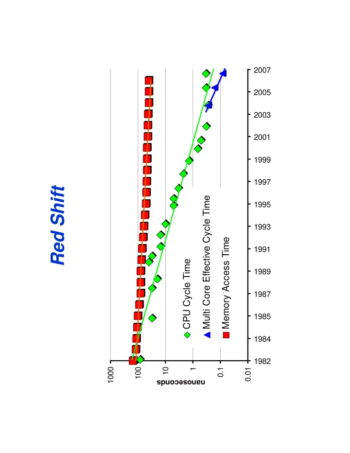
Red Shift Multi Core Effective Cycle Time 1995 1993 Memory Access - - PDF document
2007 2005 2003 2001 1999 1997 Red Shift Multi Core Effective Cycle Time 1995 1993 Memory Access Time 1991 CPU Cycle Time 1989 1987 1985 1984 1982 1000 1000 100 10 1 0.1 0.01 anoseconds na Because of Red Shift Todays
1000 100 1000 1 10 anoseconds
0.1 na
0.01 1982 1984 1985 1987 1989 1991 1993 1995 1997 1999 2001 2003 2005 2007
Skamarock W S 2004: Evaluating Mesoscale NWP Models Using Skamarock, W. S., 2004: Evaluating Mesoscale NWP Models Using Kinetic Energy Spectra. Mon. Wea. Rev., 132, 3019--3032.
http://www.wrf-model.org
5 day global WRF forecast at 20km horizontal resolution. running at 4x real time 128 processors of IBM Power5+ 128 processors of IBM Power5+ (blueice.ucar.edu)
L1 Cache
WRF large 256
1.5 L2 Cache Off-Node BW
WRF large 512
0.5 L3 Cache Off-Node Lat
tuning
Main Memory On-Node BW On-Node Lat
N.H. Real Data Forecast 20k Gl b l WRF 20km Global WRF July 22, 2007
5k (id li d) S.H. 5km (idealized) Capturing large scale structure already (Rossby Waves) Small scale features spinning up (next slide)
k-3
At 3:30 h into the simulation, the mesoscales are still spinning up and filling in the spectrum. Large scales were previously spun up
k-5/3
The cubed-sphere mapping of the globe represents a mesh
SAN DIEGO SUPERCOMPUTER CENTER at the UNIVERSITY OF CALIFORNIA, SAN DIEGO
SAN DIEGO SUPERCOMPUTER CENTER at the UNIVERSITY OF CALIFORNIA, SAN DIEGO
SAN DIEGO SUPERCOMPUTER CENTER at the UNIVERSITY OF CALIFORNIA, SAN DIEGO
SAN DIEGO SUPERCOMPUTER CENTER at the UNIVERSITY OF CALIFORNIA, SAN DIEGO
Total Disk S pace Used for All C ores
1.E +09 1.E +08 Dis k S pace (K B ) Measured Model 1.E +06 1.E +07 100 200 300 400 500 600 700 D
SAN DIEGO SUPERCOMPUTER CENTER at the UNIVERSITY OF CALIFORNIA, SAN DIEGO
100 200 300 400 500 600 700 S imulation Res olution
1.5 L1 Cache SPECFEM3D Med 54 SPECFEM3D Lrg 384 1.5 L1 Cache
SPECFEM3D Med 54 SPECFEM3D Lrg 384
L2 Cache Off-Node BW L2 Cache Off-Node BW 0.5 L3 Cache Off-Node Lat 0.5 L3 Cache Off-Node Lat Main M emory On-N
On-Node BW Main Memory On-Node Lat On-Node BW
SAN DIEGO SUPERCOMPUTER CENTER at the UNIVERSITY OF CALIFORNIA, SAN DIEGO
SAN DIEGO SUPERCOMPUTER CENTER at the UNIVERSITY OF CALIFORNIA, SAN DIEGO