Rectangle ------- ------- Rule ------- ------- . . . . ------- - - PDF document

Numerical Integration Introduction There are two types of integrals: indefinite integral and definite integral. If we can find an anti-derivative F(x) of a function f, and F is an elementary function, then we can compute I =

b

a f(x)dx = F(b) − F(a).

Maple and Mathematica can do symbolic integration (when possible). However often it is not possible to obtain such an F(x) for f(x). e.g. the case of f(x) = e−x2. When symbolic integration is not feasible, we can use numerical integration, to approximate an integral by something which is much easier to compute. One important interpretation for the definite integral

b

a f(x)dx is it is the area between

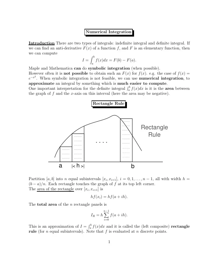
the graph of f and the x-axis on this interval (here the area may be negative). Rectangle Rule

. . . . a b

|< h >|

Rectangle Rule

• ........

........ ........

• Partition [a, b] into n equal subintervals [xi, xi+1], i = 0, 1, . . . , n − 1, all with width h =

(b − a)/n. Each rectangle touches the graph of f at its top left corner. The area of the rectangle over [xi, xi+1] is hf(xi) = hf(a + ih). The total area of the n rectangle panels is IR = h

n−1

• i=0

f(a + ih). This is an approximation of I =

b

a f(x)dx and it is called the (left composite) rectangle

rule (for n equal subintervals). Note that f is evaluated at n discrete points. 1

Error Analysis of the Rectangle Rule Tools for error analysis: The Mean-Value-Theorem

• for sum: Let q(x) be continuous on [a, b]. If p(zi) ≥ 0 for i = 1, . . ., n, then

n

• i=1

p(zi)q(zi) = q(z)

n

• i=1

p(zi), some z ∈ [a, b],

• for integrals: Let q(x) and p(x) be continuous with p(x) ≥ 0. Then

b

a p(x)q(x)dx = q(z)

b

a p(x)dx, some z ∈ [a, b]

Theorem: Let f ′ be continuous on [a, b]. Then for some z ∈ [a, b], I − IR = 1 2(b − a)hf ′(z) = O(h). Proof: We first show when h = b − a, it is true, i.e., I − IR = 1 2(b − a)2f ′(z), for some z ∈ [a, b] (∗) For every x ∈ [a, b], the Taylor series expansion gives f(x) = f(a) + (x − a)f ′(zx), for some zx ∈ [a, b]. Then I − IR =

b

a f(x)dx − f(a)(b − a)

=

b

a f(x)dx −

b

a f(a)dx

=

b

a [f(x) − f(a)]dx

=

b

a (x − a)f ′(zx)dx

= f ′(z)

b

a (x − a)dx (MVT for integral)

= 1 2(b − a)2f ′(z). Now let [a, b] be divided into n equal subintervals by x0, x1, . . . , xn with spacing h = (b − a)/n. Applying (∗) to subinterval [xi, xi+1], we have

xi+1

xi

f(x)dx − f(xi)h = (xi+1 − xi)2 2 f ′(zi) = h2 2 f ′(zi), 2

for some zi ∈ [xi, xi+1]. So we have I − IR =

b

a f(x)dx − h n−1

• i=0

f(xi) =

n−1

• i=0

xi+1

xi

f(x)dx − h

n−1

• i=0

f(xi) =

n−1

• i=0

1 2h2·f ′(zi) = f ′(z)· 1 2nh2 (MVT for sum) = 1 2(b − a)hf ′(z). Midpoint Rule

...... ...... ...... ...... ......

....... ....... ....... .

...... ...... ...... ...... ...... ......

a b

|< h >|

Midpoint Rule

, We make the midpoint of the top of each rectangle intersect the graph. The midpoint rule: IM = h

n−1

• i=0

f[a + (i + 1/2)h], where h = b − a n . Since part of the rectangle usually lies above the graph of f and part below, the midpoint rule is more accurate than the rectangle rule. It can be proven that for some z ∈ [a, b] I − IM = 1 24(b − a)h2f ′′(z) = O(h2). (Try to prove it by yourself) 3

Trapezoid Rule Consider trapezoid-shaped panels:

Trapezoid Rule a a+h a+2h . . .

The trapezoid rule: IT = 1 2h[f(a) + f(b)] + h

n−1

• i=1

f(a + ih), with h = b − a n . It can be shown that for some z ∈ [a, b] I − IT = − 1 12(b − a)h2f ′′(z) = O(h2). Q Prove both the midpoint and trapezoid rules give the exact integral if f is linear. Recursive Trapezoid Rule Suppose [a, b] is divided into 2n equal subintervals. Then the trapezoid rule is IT(2n) = 1 2h[f(a) + f(b)] + h

2n−1

• i=1

f(a + ih). where h = (b − a)/2n. The trapezoid rule for 2n−1 equal subintervals is IT(2n−1) = 1 2 ˜ h[f(a) + f(b)] + ˜ h

2n−1−1

• i=1

f(a + i˜ h). 4

where ˜ h = (b − a)/2n−1 = 2h. It is easy to show the following recursive formula IT(2n) = 1 2IT(2n−1) + h

2n−1

• i=1

f[a + (2i − 1)h]. After computing IT(2n−1) we can compute IT(2n) by this recursive formula without reeval- uating f at the old points. Simpson’s Rule There is no need for straight edges:

Simpson’s Rule a a+h a+2h . . .

Each panel is topped by a parabola. There are an even number of panels with width h = (b − a)/n. The top boundary of the first pair of panels is the quadratic which interpolates (a, f(a)), (a + h, f(a + h)), (a + 2h, f(a + 2h)). The next interpolates (a + 2h, f(a + 2h)), (a + 3h, f(a + 3h)), (a + 4h, f(a + 4h)), and so on. The area of the first 2 panels can be shown to be h 3 [f(a) + 4f(a + h) + f(a + 2h)] Q: How would you obtain this ?? Summing the areas of the pairs h 3[f(a) + 4f(a + h) + f(a + 2h)], h 3[f(a + 2h) + 4f(a + 3h) + f(a + 4h)], · · · · · ·· · · h 3[f(b − 2h) + 4f(b − h) + f(b)], 5

leads to Simpson’s rule (h = b−a

n ):

IS = h 3[f(a) + 4f(a + h) + 2f(a + 2h) + 4f(a + 3h) + · · · +4f(b − 3h) + 2f(b − 2h) + 4f(b − h) + f(b)]. It can be shown for some z ∈ [a, b] I − IS = − 1 180(b − a)h4f (4)(z) = O(h4). Q: What is the highest degree polynomial for which the rule is exact in general ?? Adaptive Simpson’s Method Motivation and ideas of an adaptive integration method: A function may varies rapidly on some parts of the interval [a, b], but varies little on other parts. It is not very efficient to use some panel width h everywhere on [a, b]. But on the other hand, it is not known in advance on which part of the integral f varies rapidly. We can consider an adaptive integration method. The basic idea is we divide [a, b] into 2 subintervals and then decide whether each of them is to be divided into more subintervals. This procedure is continued until some specified accuracy is obtained throughout the whole interval [a, b]. A framework of an adaptive method: function numI = adapt(f, a, b, ǫ, · · ·) Compute the integral from a and b in two ways and call the values I1 and I2 (assume I2 is better than I1) Estimate the error in I2 based on |I2 − I1| if |the estimated error| ≤ ǫ, then numI = I2 (or numI = I2 + the estimated error) else c = (a + b)/2 numI = adapt(f, a, c, ǫ/2, · · ·) +adapt(f, c, b, ǫ/2, · · ·) end This will guarantee |I − numI| < ∼ ǫ. Now we want to fill in details for Simpson’s method. 6

• Defining I1 and I2:

Simpson’s rule for n = 2 gives I = I1 + E1, where I1 = b − a 6 [f(a) + 4f(a + b 2 ) + f(b)], E1 = − 1 180(b − a)(b − a 2 )4f (4)(z). Simpson’s rule for n = 4 gives I = I2 + E2, where I2 = b − a 12 [f(a) + 4f(a + b − a 4 ) +2f(a + b − a 2 ) + 4f(a + 3(b − a) 4 ) + f(b)], E2 = − 1 180(b − a)(b − a 4 )4f (4)(˜ z).

• Estimating the error in I2:

We assume f (4)(z) in E1 is equal to f 4(˜ z) in E2. (a reasonable assumption if f (4) does not vary much on [a, b]). Then we observe E1 = 16E2. Since I = I1 + E1 = I2 + E2, we have I2 − I1 = E1 − E2 = 16E2 − E2 = 15E2. This gives an error estimate in I2: E2 = 1 15(I2 − I1). 7

Adaptive Simpson’s algorithm: function numI = adapt simpson(f, a, b, ǫ, level, level max) h ← b − a c ← (a + b)/2 I1 ← h[f(a) + 4f(c) + f(b)]/6 level ← level + 1 d ← (a + c)/2 e ← (c + b)/2 I2 ← h[f(a) + 4f(d) + 2f(c) + 4f(e) + f(b)]/12 if level ≥ level max, then numI ← I2 else if |I2 − I1| ≤ 15ǫ, then numI ← I2 (or numI ← I2 + 1

15(I2 − I1))

else numI ← adapt simpson(f, a, c, ǫ/2, level, level max) +adapt simpson(f, c, b, ǫ/2, level, level max) end end 8

Gaussian Quadrature Rules Unlike previous (composite) integration rules which choose equally spaced nodes for evalua- tion, Gaussian quadratiure rules choose the nodes x0, x1, . . . , xn and coefficients A0, A1, . . . , An (which are also called weights) to minimize the expected error obtained in the approxima- tion

b

a f(x)dx ≈ n

• i=0

Aif(xi). To measure this accuracy, we assume that the best choice of these values is that which produces the exact result for the largest class of polynomials.

• Theorem. Let q be a nontrival polynomial of degree n + 1 such that

b

a xkq(x)dx = 0,

k = 0, 1, . . ., n. (1) Let x0, x1, . . . , xn be the zeros of q. Then

b

a f(x)dx = n

• i=0

Aif(xi), Ai =

b

a li(x)dx,

li(x) = Πn

j=0,j=i

x − xj

xi − xj

• ,

for any polynomial f(x) with degree less than or equal to 2n + 1. Any IG =

n

i=0 Aif(xi) with xi and Ai (i = 0, 1, . . .n) defined as in the above theorem

called a Gaussian quadrature rule. If the interval [a, b] = [−1, 1], the Legendre polynomial qn+1(x) defined by qn+1(x) = 2n + 1 n + 1 xqn(x) − n n + 1qn−1(x), q0(x) = 1, q1(x) = x. satisfies (1). Thus the roots of qn+1(x) = 0 are the nodes of the Gaussian quadrature rule for

1

−1 f(x)dx.

If the Gaussian quadrature rule for

1

−1 f(x)dx is IG[−1, 1] =

n

i=0 Aif(xi). Then it can

shown that the Gaussian quadrature rule for

b

a f(x)dx is

IG[a, b] = β

n

• i=0

Aif(α + βxi), α = 1 2(a + b), β = 1 2(b − a). 9