Recall: Antialiasing Raster displays have pixels as rectangles - - PowerPoint PPT Presentation

Recall: Antialiasing

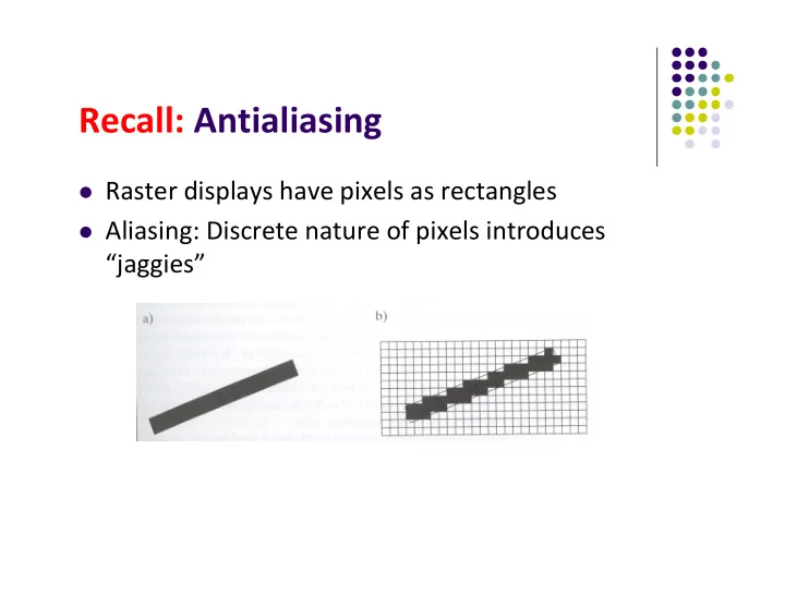
 Raster displays have pixels as rectangles  Aliasing: Discrete nature of pixels introduces

“jaggies”

Recall: Antialiasing

 Aliasing effects:

 Distant objects may disappear entirely  Objects can blink on and off in animations

 Antialiasing techniques involve some form of

blurring to reduce contrast, smoothen image

 Three antialiasing techniques:

 Prefiltering  Postfiltering  Supersampling

Prefiltering

 Basic idea:

 compute area of polygon coverage  use proportional intensity value

 Example: if polygon covers ¼ of the pixel

 Pixel color = ¼ polygon color + ¾ adjacent region color

 Cons: computing polygon coverage can be time

consuming

Supersampling

 Assumes we can compute color of any location (x,y) on screen  Sample (x,y) in fractional (e.g. ½) increments, average samples  Example: Double sampling = increments of ½ = 9 color values

averaged for each pixel

Average 9 (x, y) values to find pixel color

Postfiltering

 Supersampling weights all samples equally  Post‐filtering: use unequal weighting of samples  Compute pixel value as weighted average  Samples close to pixel center given more weight

1 / 2 1 / 1 6 1 / 1 6 1 / 1 6 1 / 1 6 1 / 1 6 1 / 1 6 1 / 1 6 1 / 1 6

Sam ple w eighting

Antialiasing in OpenGL

 Many alternatives  Simplest: accumulation buffer  Accumulation buffer: extra storage, similar to frame

buffer

 Samples are accumulated  When all slightly perturbed samples are done, copy

results to frame buffer and draw

Antialiasing in OpenGL

 First initialize:  glutInitDisplayMode(GLUT_SINGLE |

GLUT_RGB | GLUT_ACCUM | GLUT_DEPTH);

 Zero out accumulation buffer  glClear(GLUT_ACCUM_BUFFER_BIT);  Add samples to accumulation buffer using  glAccum( )

Antialiasing in OpenGL

 Sample code  jitter[] stores randomized slight displacements of camera,  factor, f controls amount of overall sliding

glClear(GL_ACCUM_BUFFER_BIT); for(int i=0;i < 8; i++) { cam.slide(f*jitter[i].x, f*jitter[i].y, 0); display( ); glAccum(GL_ACCUM, 1/8.0); } glAccum(GL_RETURN, 1.0); jitter.h

• 0.3348, 0.4353

0.2864, -0.3934 … …

Computer Graphics CS 4731 Lecture 26 Curves Prof Emmanuel Agu

Computer Science Dept. Worcester Polytechnic Institute (WPI)

So Far…

 Dealt with straight lines and flat surfaces  Real world objects include curves  Need to develop:

 Representations of curves (mathematical)  Tools to render curves

Interactive Curve Design

 Mathematical formula unsuitable for designers  Prefer to interactively give sequence of points

(control points)

 Write procedure:

 Input: sequence of points  Output: parametric representation of curve

Interactive Curve Design

 1 approach: curves pass through control points (interpolate)  Example: Lagrangian Interpolating Polynomial  Difficulty with this approach:



Polynomials always have “wiggles”



For straight lines wiggling is a problem

 Our approach: approximate control points (Bezier, B‐Splines)

De Casteljau Algorithm

 Consider smooth curve that approximates sequence

• f control points [p0,p1,….]

 Blending functions: u and (1 – u) are non‐negative

and sum to one

1

) 1 ( ) ( up p u u p    1   u

System generates this point using math Artist provides these points

 Now consider 3 points  2 line segments, P0 to P1 and P1 to P2

De Casteljau Algorithm

1 01

) 1 ( ) ( up p u u p   

2 1 11

) 1 ( ) ( up p u u p   

De Casteljau Algorithm

) ( ) 1 ( ) (

11 01

u up p u u p   

2 2 1 2

)) 1 ( 2 ( ) 1 ( p u p u u p u     

2 02

) 1 ( ) ( u u b  

Blending functions for degree 2 Bezier curve

) 1 ( 2 ) (

12

u u u b  

2 22

) ( u u b 

) (

02 u

b ) (

12 u

b

) (

22 u

b

Substituting known values of and

) (

01 u

p

) (

11 u

p

Note: blending functions, non-negative, sum to 1

De Casteljau Algorithm

 Extend to 4 control points P0, P1, P2, P3  Final result above is Bezier curve of degree 3

3 2 2 1 2 3

)) 1 ( 3 ( ) ) 1 ( 3 ( ) 1 ( ) ( u p u u p u u p u u p        ) (

23 u

b ) (

03 u

b ) (

13 u

b ) (

33 u

b

De Casteljau Algorithm

 Blending functions are polynomial functions called

Bernstein’s polynomials

3 33 2 23 2 13 3 03

) ( ) 1 ( 3 ) ( ) 1 ( 3 ) ( ) 1 ( ) ( u u b u u u b u u u b u u b       

3 2 2 1 2 3

)) 1 ( 3 ( ) ) 1 ( 3 ( ) 1 ( ) ( u p u u p u u p u u p        ) (

23 u

b ) (

03 u

b ) (

13 u

b ) (

33 u

b

Subdividing Bezier Curves

 OpenGL renders flat objects  To render curves, approximate with small linear

segments

 Subdivide surface to polygonal patches  Bezier Curves can either be straightened or curved

recursively in this way

Bezier Surfaces

 Bezier surfaces: interpolate in two dimensions  This called Bilinear interpolation  Example: 4 control points, P00, P01, P10, P11,



2 parameters u and v

 Interpolate between



P00 and P01 using u



P10 and P11 using u



P00 and P10 using v



P01 and P11 using v

) ) 1 (( ) ) 1 )(( 1 ( ) , (

11 10 01 00

up p u v up p u v v u p       

Problems with Bezier Curves

 Bezier curves elegant but to achieve smoother curve

 = more control points  = higher order polynomial  = more calculations

 Global support problem: All blending functions are

non‐zero for all values of u

 All control points contribute to all parts of the curve  Means after modelling complex surface (e.g. a ship), if

• ne control point is moves, recalculate everything!

B‐Splines

 B‐splines designed to address Bezier shortcomings  B‐Spline given by blending control points  Local support: Each spline contributes in limited range  Only non‐zero splines contribute in a given range of u







m i i i

p u B u p ) ( ) (

B-spline blending functions, order 2

NURBS

 Non‐uniform Rational B‐splines (NURBS)  Rational function means ratio of two polynomials  Some curves can be expressed as rational functions but not as

simple polynomials

 No known exact polynomial for circle  Rational parametrization of unit circle on xy‐plane:

) ( 1 2 ) ( 1 1 ) (

2 2 2

      u z u u u y u u u x

Tesselation

 Previously: Pre‐generate mesh versions offline  Tesselation shader unit new to GPU in DirectX 10 (2007)



Subdivide faces on‐the‐fly to yield finer detail, generate new vertices, primitives

 Mesh simplification/tesselation on GPU = Real time LoD

tesselation Simplification

Far = Less detailed mesh Near = More detailed mesh

Tessellation Shaders

 Can subdivide curves, surfaces on the GPU

Where Does Tesselation Shader Fit?

Fixed number of vertices in/out Can change number of vertices

Geometry Shader

 After Tesselation shader. Can

 Handle whole primitives  Generate new primitives  Generate no primitives (cull)

References

 Hill and Kelley, chapter 11  Angel and Shreiner, Interactive Computer Graphics,

6th edition, Chapter 10

 Shreiner, OpenGL Programming Guide, 8th edition

Computer Graphics (CS 4731) Lecture 26: Image Manipulation Prof Emmanuel Agu

Computer Science Dept. Worcester Polytechnic Institute (WPI)

Image Processing

 Graphics concerned with creating artificial scenes

from geometry and shading descriptions

 Image processing

 Input is an image  Output is a modified version of input image

 Image processing operations include altering images,

remove noise, super‐impose images

Image Processing

 Example: Sobel Filter

 Image Proc in OpenGL: Fragment shader invoked on each

element of texture



Performs calculation, outputs color to pixel in color buffer

Original Image Sobel Filter

Luminance

 Luminance of a color is its overall brightness (grayscale)  Compute it luminance from RGB as

Luminance = R * 0.2125 + G * 0.7154 + B * 0.0721

Image Negative

 Another example

Edge Detection

 Edge Detection

 Compare adjacent pixels

 If difference is “large”, this is an edge  If difference is “small”, not an edge

 Comparison can be done in color or luminance Insert figure 11.11

Embossing

 Embossing is similar to edge detection  Replace pixel color with grayscale proportional to contrast

with neighboring pixel

 Add highlights depending on angle of change

Insert figure 11.12

Toon Rendering for Non‐Photorealistic Effects

Geometric Operations

 Examples: translating, rotating, scaling an image

Non‐Linear Image Warps

Original Twirl Ripple Spherical

References

 Mike Bailey and Steve Cunningham, Graphics Shaders (second

edition)

 Wilhelm Burger and Mark Burge, Digital Image Processing: An

Algorithmic Introduction using Java, Springer Verlag Publishers

 OpenGL 4.0 Shading Language Cookbook, David Wolff  Real Time Rendering (3rd edition), Akenine‐Moller, Haines and

Hoffman

 Suman Nadella, CS 563 slides, Spring 2005

Computer Graphics CS 4731 – Final Review Prof Emmanuel Agu

Computer Science Dept. Worcester Polytechnic Institute (WPI)

Exam Overview

 Thursday, October 16, 2014 in‐class  Midterm covered up to lecture 13 (Viewing & Camera Control)  Final covers lecture 14 till today’s class (lecture 26)  Can bring:  1 page cheat‐sheet, hand‐written (not typed)  Calculator  Will test:  Theoretical concepts  Mathematics  Algorithms  Programming  OpenGL/GLSL knowledge (program structure and commands)

Topics

 Projection  Lighting, shading and materials  Shadows and fog  Texturing & Environment mapping  Image manipulation  Clipping (2D and 3D clipping) and viewport

transformation

 Hidden surface removal  Rasterization (line drawing, polygon filling, antialiasing)  Curves