Real-Time Communication Integrated Services: Integration of - - PDF document

CPSC-663: Real-Time Systems Real-Time Communication 1

Real-Time Communication

• Integrated Services: Integration of variety of services with

different requirements (real-time and non-real-time)

• Traffic (workload) characterization
• Scheduling mechanisms
• Admission control / Access control (policing)
• Deterministic vs. stochastic analysis

– Traffic characterization – Performance guarantees

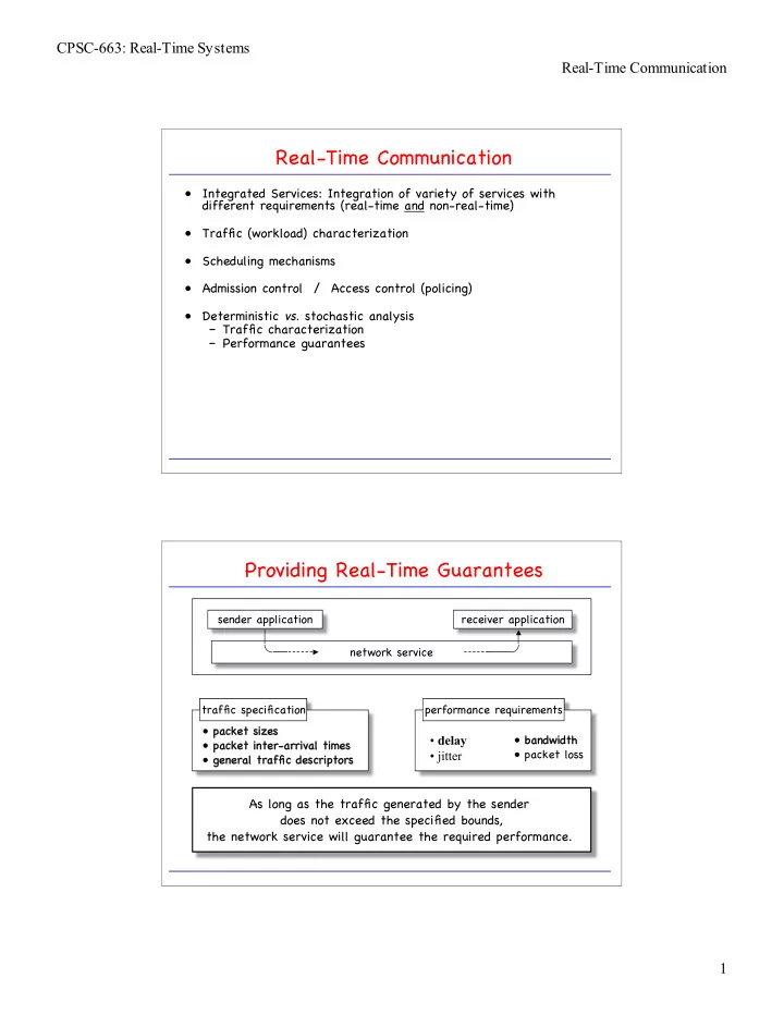
performance requirements traffic specification

Providing Real-Time Guarantees

network service sender application receiver application

• packet sizes
• packet inter-arrival times
• general traffi

fic descriptors

• delay
• jitter
• bandwidth
• packet loss

As long as the traffic generated by the sender does not exceed the specified bounds, the network service will guarantee the required performance.

CPSC-663: Real-Time Systems Real-Time Communication 2

network service

Real-Time Guarantees: Mechanisms

sender application receiver application deterministic packet scheduling in switches and routers Enforcement:

• policing
• traffic shaping

connection-oriented service rigorous (and robust) delay computation real-time-connection establishment

Traffic Description: Traffic Bounding Functions

• Arrival as stochastic process

A = {A(t), t ≥ 0}

• A and a are poor traffic descriptors:

– time dependent

• Deterministic traffic arrival descriptors (time-independent)

– Maximum Traffi fic Function b(I) ≥ maxt>0{A(t+I) – A(t)} – Maximum Rate Function b(I)/I ≥ maxt>0{A(t+I) – A(t)}/I

t

rate [b/sec]

A(t)

a(t)

CPSC-663: Real-Time Systems Real-Time Communication 3

Maximum Traffic Functions

Time Interval [msec]

20 40 60 80 100 120 140 1 10 100 1,000 10,000 100,000

• Max. Data Rate [Mb/sec]

Peak Rate Average Rate

• bserved max.

rate function b(I)/I

I b(I)/I I t A I t A I I b

t

/ )) ( ) ( ( max / ) ( − + =

≥

Traffic Bounding Functions

Time Interval [msec]

20 40 60 80 100 120 140 1 10 100 1,000 10,000 100,000

• Max. Data Rate [Mb/sec]

Peak Rate Average Rate

• bserved max.

rate function b(I)/I Peak-Rate Leaky Bucket Pair

I b(I)/I

CPSC-663: Real-Time Systems Real-Time Communication 4

Maximum Rate vs. Maximum Traffic Functions

Maximum Rate Representation

b(I)/I I b(I)/I I

Maximum Traffic Representation

b(I) I b(I) I I1 I2 I1 I2

Traffic Models

Deterministic:

• 1. Periodic model: (e, p)
• 2. Deferred Server, Sporadic Server model: (eS, pS)
• 3. (σ, ρ) model [Cruz]
• 4. Leaky bucket model [Turner, ...]: (β, ρ)
• 5. (xmin, xave, I, smax) model [Ferrari & Verma]
• 6. D-BIND model (Deterministic Bounding Interval Length Dependent)

[Knightly & Zhang]

• 7. Γ-functions [Zhao]

Probabilistic:

• 1. S-BIND model (Stochastic Bounding Interval) [Knightly]
• 2. Markov-Modulated Poisson Processes

CPSC-663: Real-Time Systems Real-Time Communication 5

Traffic Bounding Function b(.)

• Let b(.) be a monotonically increasing function.
• b(.) is a deterministic traffic constraint function of a connection

if during any interval of length I, the number of bits arriving during the interval is no greater than b(I).

• Let A[t1,t2] be the number of packets arriving during interval

[t1,t2]. Then, b(.) is a traffic constraint function if

• Each model defines inherently a traffic constraint function.
• The accuracy of models can be compared by comparing their

constraint functions.

Cruz’ (σ, ρ) Model

• If the traffic is fed to a server that works at rate ρ while there is

work to be done, the size of the backlog will never be larger than σ.

• IOW:

The number of jobs/cells released during any interval I does not exceed ρI+σ.

• Graphical representation:

I worst case number b(.)

• f jobs/cells released

σ ρ

CPSC-663: Real-Time Systems Real-Time Communication 6

The Leaky Bucket Model

• Implementation:

– Maintain counter for each traffic stream. – Increment counter at rate ρ, to maximum of β. – Each time a packet is

• ffered, the counter is

checked to be > 0. – If so, decrement counter and forward packet; otherwise drop packet.

β ρ data

I

worst case number of jobs/cells released

β ρ

Concatenating Leaky Buckets

• What about limiting the maximum cell rate?

β1 ρ1 data β2=1 ρ2

x worst case number of jobs/cells released

β1 ρ1

ρ2

β2

CPSC-663: Real-Time Systems Real-Time Communication 7

(xmin, xave, Iave, smax) model [Ferrari & Verma]

• xmin : minimum packet interarrival time
• xave : average packet interarrival time
• Iave

: averaging interval length

• smax : maximum packet length

I

worst case number of jobs/cells released

1/xave 1/xmin Iave

max min max min

, mod min ) )( , , , ( s I I x I x I t I s I x x b

ave ave ave ave ave ave

        +                     =

D-BIND [Knightly & Zhang]

• Other models do not accurately describe burstiness.
• Rate-interval representation:

interval length [sec] bounding rate [Mbps] long-term average rate 1.6 0.5 1.0 lecture advertisements

• Model traffic by multiple rate-interval pairs: (Rk, Ik), where rate Rk is

the worst-case rate over every interval of length Ik.

CPSC-663: Real-Time Systems Real-Time Communication 8

D-BIND (2)

• Constraint function for D-BIND model with P rate-interval pairs:
• Comparison:

interval length D-BIND (σ, ρ) xmin, ... maximum bits

 

P P k k k k k k k k k k k

I t I t t b t b b I t I I R I t I I I R I R t b > − = = ≤ ≤ + − − − =

− − − −

for ) / ( ) ( ) ( , ) ( ) (

1 1 1 1

Policing for the D-BIND Model

• Lemma:

If b(t) is piece-wise linear concave, then Rk is strictly decreasing with increasing Ik.

• Lemma:

If a piece-wise linear constraint function b(t) with P linear segments is concave, then the source may be fully policed with a cascade of P leaky buckets.

link rate concave hull

CPSC-663: Real-Time Systems Real-Time Communication 9

Delay Computation: Overview

• Delay computation for FIFO server with deterministically

constraint input traffic:

R

b1(I) b2(I) b1(I)+b2(I)

R RI I b d

i i I FIFO

/ ) ( max       − =

∑

>

End-to-End Analysis

• Traffic regulation: reshape traffic to adhere to traffic function.
• Alternative: re-characterize by accounting for burstiness added by

queueing delays FY(I) = FX(I+dY)

– where dY is delay on Server Y.

• Deterministic Case:

X Y FX(I) FY(I)

CPSC-663: Real-Time Systems Real-Time Communication 10

Switch Scheduling

• Work-conserving (greedy) vs. non-work-conserving (non-greedy)

mechanisms.

• Rate-allocating disciplines: Allow packets to be served at higher

rates than the guaranteed rate.

• Rate-controlled disciplines: Ensures each connection the

guaranteed rate, but does not allow packets to be served above guaranteed rate.

• Priority-based scheduling:

– fair queuing – virtual clock – earliest due date (EDD) – rate-controlled static priority (RCSP)

• Weighted Round-Robin scheduling:

– WRR

Bit-by-Bit Weighted Round-Robin

• bit-by-bit round robin
• each connection is given

a weight

• each queue served in

FIFO order wi

CPSC-663: Real-Time Systems Real-Time Communication 11

Fair Queueing [Demers, Keshav, Shenker]

• Emulate Bit-by-Bit Round Robin by prioritizing packets.
• Prioritize packets on basis of their finish time fj:

– aj: arrival time of j-th packet – ej: length of packet – fj: finish time – BW: allocated fraction of link bandwidth

• Example:
• Complications:

– What if connections dynamically change?

1 4 1.5 1 1 BW e a f f

j j j j

/ ) , max(

1

+ =

−

Virtual Clock Algorithm [L.Zhang]

• Emulate time-division multiplex (TDM) mechanism
• However:

– TDM: when some connections idle, the slots assigned are idle – VC: idle slots are deleted from TDM frames

• auxiliary virtual clock (auxVCj): finish time of j-th packet.
• virtual tick (Vtickj) :time to complete transmission of ready j-th

packet. Vtickj = ej/BW

• Replace fj by Vtickj: VC becomes identical to WFQ algorithm!
• Will analyze delay analysis later.

CPSC-663: Real-Time Systems Real-Time Communication 12

Rate-Controlled Static Priority (RCSP) [Zhang&Ferrari]

priority queues

RCSP (2)

rate controller priority queues

CPSC-663: Real-Time Systems Real-Time Communication 13

Traffic Regulation in RCSP

• Hold packets in regulator to guarantee minimum inter-packet

arrival time. ri,j = max(ai,j, ri,j-1+pi)

• Implementation:

buffer and timers in traffic regulator.

• Buffer requirements:

rate controller priority queues

i i ik i ik ik

e p d p d B ) (

1 

     +       =

−

Is it Necessary to Regulate?

• [Liebeherr, Wrege, Ferrari, Transactions on Networking, 1995]
• Generalization of schedulability for arbitrary traffic constraint functions

b(I):

Theorem: A set N of connections that is given by {bj, dj} is schedulable according to a static-priority algorithm if and only if for all priorities p, and for all I >= 0 there is a t with t <= dp - sp

min

such that:

{ }

max 1 1 min min

max ) ) (( ) ( : ,

r p r p q C j j p C j j p p

s t I b s I b t I s d t I

q p

> − = ∈ − ∈

+ + + − ≥ + − ≤ ∃ ∀

∑ ∑ ∑

CPSC-663: Real-Time Systems Real-Time Communication 14

Earliest Due Date (EDD) [Ferrari]

• based on EDF
• delay-EDD vs. jitter-EDD
• works for periodic message models (single packet in period): (pi, 1, Di)
• partition end-to-end deadline Di into local deadlines Di,k during connection

establishment procedure.

• 2-Phase establishment procedure:

Sender Receiver OK? Sender Receiver Fine!

Phase 1: tentative establishment Phase 2: relaxation

Delay EDD

• Upon arrival of Packet j of Connection i:

– Determine effective arrival time: ae

i,j = max(ae i,j-1 + pi, ai,j)

– Stamp packet with local deadline: di,j = ae

i,j + Di,k

– Process packets in EDF order.

• Delay EDD is greedy.
• Can be mapped into special case of Sporadic Server.
• Acceptance test (Δ = total density): Δ + 1/pi < 1 - 1/pmin
• Offered local deadline: LDi = min(pi, 1/(1-Δ-1/pmin))
• Problem with EDD: jitter

– max end-to-end delay over k switches: – min end-to-end delay over k switches: k

∑

k k i

D ,

CPSC-663: Real-Time Systems Real-Time Communication 15

Jitter EDD

• Problem with Delay-EDD: does not control jitter. This has effect
• n buffer requirements.
• Jitter-EDD maintains Ahead Time ahi,j, which is the difference

between local relative deadline Di,k-1 and actual delay at Switch k-1.

• Ahead time is stored in packet header (alternatively, we use

global time synchronization)

• Upon receiving the j-th packet of Connection i with ahi,j at time

ai,j: – Calculate ready time as Switch k: ae

i,j=max(ae i,j-1 + pi , ai,j)

ri,j = max(ae

i,j , ai,j + ahi,j)

– Stamp packet with deadline di,j=ri,j+Di,k and process according to EDF starting from ready time ri,j.

• Result: Regenerate traffic at each switch.

Rate Control vs. Jitter Control

• Rate Control
• Jitter Control

CPSC-663: Real-Time Systems Real-Time Communication 16

Simple EDF with Arbitrary Arrival Functions

[Liebeherr, Wrege, Ferrari: Transactions on Networking, 1995] Theorem: A set Π of connections that is given by {bi; di} iεΠ and di ≤ dj whenever i<j is EDF schedulable if and only if for all I ≥ d1: where Informal “proof”: A deadline violation occurs at time I if the maximum traffic arrivals with deadline before or at time I, i.e. exceeds I.

{ }

∑

Π ∈ >

+ − ≥

j k I d k j j

s d I b I

k

max ,

max ) (

{ } { }

k k k I d k

d I for , s

k

Π ∈ >

> ≡ max max

max ,

∑

Π ∈

− <

j j j

d I b I ) (

• For some traffic models, closed-form expressions for the

schedulability test exist.

• For (σ, ρ) traffic:
• A closed form for the delay can be given as follows:

EDF Test for Special Cases: Example (σ,ρ)

{ }

       ≥ − + ≥ Π < ≤ < ≤ + − + ≥

Π Π = + > =

∑ ∑

d I d I I j d I d s d I I

i i i i j j k j k j i i i i

for ) ( 1 : for max ) (

1 1 max 1

ρ σ ρ σ

{ }

∑ ∑

− = − = >

− + − + =

1 1 1 1 max

1 max ) (

j i i j i k j k i i i j j

s d d ρ ρ σ σ

CPSC-663: Real-Time Systems Real-Time Communication 17

Weighted Round Robin (WRR)

• Traffic model:

– periodic (pi, ei, Di) – variable bit rate models possible

• Realizations:

– greedy WRR – Stop-and-Go (SG) – Hierarchical Round Robin (HRR)

• Each connection i is assigned

a weight wi, i.e., it is allocated wi slots during each round.

• Slot: time to transmit

maximum-sized packet.

wi

Throughput and Delay Guarantees

• Each connection i is guaranteed wi slots in each rounds.
• Round length RL : upper bound on sum of weights (design parameter)
• Constraints:

1. 2.

• Delays:

– at first switch: – downstream: once packet passes first switch, it is immediately eligible on switches downstream -> has to wait at most RL => end-to-end delay through N switches:

RL p ≤

min

 

     ≥ RL p e w

i i i

w RL

i ≤

∑

RL w e

i i 

    

 

( )

RL N p RL N w e W

i i i i

) 1 ( 1 − + ≤ − + ≤

CPSC-663: Real-Time Systems Real-Time Communication 18

• Greedy WRR does not control jitter:
• min end-to-end delay:

ei +(N-1)

• max end-to-end delay:

pi +(N-1)RL

• jitter:

pi-ei +(N-1)(RL-1)

• Buffer needed at k-th switch for Connection i:
• Need traffic shaping at each switch.

Problems with Greedy WRR

 

i i

e p RL k ) / ) 1 )( 1 ( 1 ( − − +

First Switch

Non-Greedy WRR

• Actual length of rounds in greedy WRR varies with amount of

traffic at switch.

• Non-greedy WRR schemes fix round length into fixed-length

frames.

• Stop-and-Go [Golestani]
• Hierarchical Round Robin [Kalmanek, K., K.]

CPSC-663: Real-Time Systems Real-Time Communication 19

Stop & Go [Golestani, 1990]

• Frame-based: divide time in frames of length RL.
• Packet arriving during frame at input link is eligible for transmission during next

frame on output link.

• Stop-and-Go is not work-conserving.
• Traffic model [(r, RL) smooth traffi

fic]: during each frame of length RL, the total number of bits transmitted by source does not exceed rRL bits.

• Proposition: If the connection satisfies (r,RL) smoothness at the input of

the first server, and each server ensures that packets will always go

• ut on the next departing frame, the connection will satisfy (r,RL)

smoothness at each server throughout the network.

input frames

• utput

frames input frames

Stop & Go: Implementation

• Implementation of scheduler is not defined by Stop-and-Go

frameworks.

• Implementation 1: FIFO scheduler with double-queue structure
• Implementation 2:

CPSC-663: Real-Time Systems Real-Time Communication 20

• Hierarchical framing with n levels with frame sizes RL1, ..., RLn, where

RLm+1=KmRLm for m = 1, ..., n-1.

• Stop-and-Go rule for packets of level-p connection: Packets that arrived

during a RLp frame will not become eligible until the start of the next RLp frame.

• Packets with smaller frame size have higher priority (non-preemptively)
• ver packets with larger frame size.

Multi-Frame Stop-and-Go

[For example, Zhang&Knightly: “Comparison of RCSP and SG”, ACM Multimedia, 4(6) 1996]

• Problem with Stop-and-Go (or any other frame-based approach): delay-

bandwidth coupling – Delay of packet is bounded by a multiple of frame time. This is a problem, for example for low-bandwidth, low-delay connections. (Why?)

• Solution: Use multi-level framing. Example:

RL1 RL2

Hierarchical Round Robin

[Kalmanek, Kanadia, Keshav, 1990]

• End-to-end delay and jitter of S&G depends on RL only.
• How about having multiple S&G servers, with different RL’s, and

multiplex them on the same outgoing link?

wi RLx swx

• Server X is seen as periodic stream of requests by Server S, with

– ex = swx, px = RLx, Dx = RLx – schedule using rate-monotonic scheduler – Configuration time test: check whether task set {(swx,RLx,RLx)} is schedulable.

• Admission Control Test:

– Bandwidth test: check sum of required wi’s <= swx – Delay test: End-to-end delay: pi + N RLx – Jitter test: 2 RLx, with buffer requirement 2 wi Server X Server S