Rate-Based Resource Allocation scheduling in particular, dominates - - PowerPoint PPT Presentation

▶

Nov 14, 2022 195 likes •282 views

Rate-Based Resource Allocation EMSOFT 2001 The case against static priority scheduling Static priority scheduling in general, and Rate Monotonic Rate-Based Resource Allocation scheduling in particular, dominates in the real-time Models for

SLIDE 1

Rate-Based Resource Allocation Models for Real-Time Computing

http://www.cs.unc.edu/Research/dirt

Kevin Jeffay

Department of Computer Science Department of Computer Science University of North Carolina University of North Carolina at Chapel Hill at Chapel Hill jeffay jeffay@ @cs cs. .unc unc. .edu edu

Steve Goddard

Computer Science & Engineering Computer Science & Engineering University of Nebraska – Lincoln University of Nebraska – Lincoln goddard goddard@ @cse cse. .unl unl. .edu edu

EMSOFT 2001

Rate-Based Resource Allocation

The case against static priority scheduling

◆ Static priority scheduling in general, and Rate Monotonic

scheduling in particular, dominates in the real-time systems literature

» VxWorks, VRTX, QNX, pSOSystems, LynxOS all support static priority scheduling

◆ Does one size fit all?

» “When you have a hammer, everything looks like a nail”

◆ Problems with static priority scheduling

» Feasibility is dependent on a predictable environment and well- behaved tasks.

Rate-Based Resource Allocation

Overview

◆ The problem:

» How to allocate resources in an environment wherein…

❖ Work arrives at well-defined but highly variable rates ❖ Tasks may exceed their execution time estimates

» … and still guarantee adherence to deadlines

◆ The thesis:

» Static priority scheduling is the wrong tool for the job (existing task models are too simplistic) » Rate-based scheduling abstractions can simplify the design and implementation of many real-time systems and improve performance and resource utilization

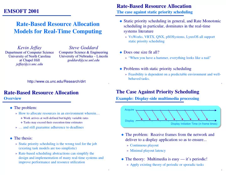
The Case Against Priority Scheduling

Example: Display-side multimedia processing

◆ The problem: Receive frames from the network and

deliver to a display application so as to ensure...

» Continuous playout » Minimal playout latency

◆ The theory: Multimedia is easy — it’s periodic!

» Apply existing theory of periodic or sporadic tasks

Acquire Display Display Initiation Time (in frame times)

SLIDE 2

Display-side Media Processing

The practice

◆ Nothing is periodic in a distributed system! ◆ The effects of distributed systems pathology:

» Variable message transmission times » Out-of-order message arrivals » Lost & duplicate messages

Acquire Display Display Initiation Time (in frame times)

X

Acquire Display Display Initiation Time (in frame times)

X

Display-side Media Processing

Managing the Network Interface

◆ Packets fragmented in the network must be

reassembled

» Messages have deadlines, packets do not » Applications know about messages, operating systems do not

The Case Against Priority Scheduling

Example: Signal processing data flow graphs

2 4 6 8 10 12 14 16 18 20 22 24 26 28 30 32 34 Time

w u

Node u has a period of 3 Node v has a period of 5

v

W U

produce = 3 t hes hol d = 7, consume = 5

V

produce = 4 t hes hol d = 4 consume = 4

Rate-Based Computing

Approaches

◆ Extend the Liu and Layland model of real-time tasks to

allow the expression of real-time rates

» Hierarchical “server-based” scheduling — Create a “server” process that is scheduled as a periodic task and internally schedules the processing of aperiodic events » Event-based scheduling — Process aperiodic events as if they were generated by a virtual “well behaved” periodic process

◆ Adapt “fluid-flow” models of resource allocation

developed in the networking community for bandwidth allocation to CPU scheduling

» Provide a “virtual processor” abstraction wherein each task logically executes on a dedicated processor with 1/ƒ(n) the capacity of the physical processor

SLIDE 3

An Event-Based Rate Model

The Rate-Based Execution (RBE) model

◆ Tasks make progress at the rate of processing x events

every y time units and each event is processed within d time units (in the best case)

◆ For task i with rate specification (xi, yi, di), the jth event

for task i, arriving at time ti,j, will be processed by time

» D(i,j) gives the earliest possible deadline for the jth instance

f task i (≥ ti,j + di)

ti,j + di if 1 ≤ j ≤ xi MAX(ti,j + di , D(i, j–xi)+yi ) if j > xi D(i, j) =

The RBE Task Model

Example: Periodic arrivals, periodic service

◆ Task with rate specification (x = 1, y = 2, d = 2)

J1,1 J1,2 J1,4 J1,5 J1,6 J1,7 J1,8 J1,9 J1,10 J1,11 J1,12

0 2 4 6 8 10 12 14 16 18 20 22 24 26

J1,3

ti,j + di if 1 ≤ j ≤ xi MAX(ti,j + di , D(i, j–xi)+yi ) if j > xi D(i, j) = » Deadlines separated by at least y = d = 2 time units » Deadlines occur at least 2 time units after a job is released

ti,j + di if 1 ≤ j ≤ xi MAX(ti,j + di , D(i, j–xi)+yi ) if j > xi D(i, j) =

The RBE Task Model

Example: Periodic arrivals, deadline ≠ period

◆ Task with rate specification (x = 1, y = 2, d = 6)

0 2 4 6 8 10 12 14 16 18 20 22 24 26 28

J1,1 J1,2 J1,3 J1,4 J1,5 J1,6 J1,7 J1,8 J1,9 J1,10 J1,11 J1,12

» Deadlines separated by at least y = 2 time units and occur at least d = 6 time units after a job is released

The RBE Task Model

Bursty arrivals

◆ Task with rate specification (x = 1, y = 2, d = 6)

» Deadlines separated by at least y = 2 time units and occur at least d = 6 time units after a job is released

0 2 4 6 8 10 12 14 16 18 20 22 24 26 28

J1,1 J1,2 J1,3 J1,4 J1,5 J1,6 J1,7 J1,8 J1,9

SLIDE 4

The RBE Task Model

Bursty arrivals

◆ Task with rate specification (x = 3, y = 6, d = 6)

» Deadlines separated by at least y = 6 time units and occur at least d = 6 time units after a job is released

0 2 4 6 8 10 12 14 16 18 20 22 24 26 28

J1,1 J1,2 J1,3 J1,4 J1,5 J1,6 J1,7 J1,8 J1,9

The RBE Task Model

Comparison of rate specifications

Rate specification (x = 1, y = 2, d = 6) Rate specification (x = 3, y = 6, d = 6)

J1,1 J1,2 J1,3 J1,4 J1,5 J1,6 J1,7 J1,8 J1,9 0 2 4 6 8 10 12 14 16 18 20 22 24 26 J1,1 J1,2 J1,3 J1,4 J1,5 J1,6 J1,7 J1,8 J1,9 0 2 4 6 8 10 12 14 16 18 20 22 24 26

The RBE Task Model

RBE features/properties

◆ Provides better response

time for non-real-time activities by integrating application-level buffering with the system run queue

Receiver’s Processing Pipeline Display Network Reception 0 2 4 6 8 10 12

Rate specification (x = 1, y = 2, d = 6)

The RBE Task Model

RBE features/properties

◆ Provides a more natural

way of modeling inbound packet processing of fragmented messages

0 2 4 6 8 10 12

Rate specification (x = 3, y = 6, d = 6)

Acquire Display

Display Initiation Time

SLIDE 5

The RBE Task Model

RBE features/properties

◆ Provides isolation from

arrival rates that exceed the rate specification

» (But does not provide isolation from tasks exceeding their stated execution time)

0 2 4 6 8 10 12

Rate specification (x = 3, y = 6, d = 6)

Acquire Display

Display Initiation Time

Fluid Flow Resource Allocation

Proportional share resource allocation

◆ Tasks are allocated a share of the processor’s capacity

» Task i is assigned a weight wi » Task i’s share of the CPU at time t is fi(t) =

◆ If tasks’ weights remain constant in [t1, t2] then task i

receives units of execution time in [t1, t2]

wi

Σj A(t) wj

∋

Si(t1,t2) = ∫ fi(t) dt = (t2 – t1)

Σj wj

wi

t1 t2

◆ Weighted round robin scheduling with an infinitesimally

small quantum

◆ In [t1, t2] (if total weight doesn’t change) Ti receives

Proportional Share Resource Allocation

Fluid scheduling example

T3: 1 0.125 T2: 1 0.125 T1: 4 0.5

Time

T4: 1 0.125 T5: 1 0.125

0 1 2 3 4 5 6 7 8 9

Weight Share

Si(t1,t2) = = ∫ fi(t) dt = (t2 – t1)

Σj A(t) wj

∋

wi

t1 t2

◆ Weighted round robin scheduling with integer quanta

» q = 1

◆ The quantum system doesn’t proportionally allocate

the resource over all time intervals

Proportional Share Resource Allocation

Quantum scheduling example

T3: 1 0.125 T2: 1 0.125 T1: 4 0.5 T4: 1 0.125 T5: 1 0.125 Weight Share

Time 0 1 2 3 4 5 6 7 8 9

SLIDE 6

◆ Schedule tasks so that their performance is as close as

possible to that in the fluid system

◆ Why is fluid allocation important?

» What about real-time allocation?!

Proportional Share Resource Allocation

Task scheduling metrics & goals

Quantum Allocation Fluid Allocation Si(t1,t2) si(t1,t2)

Approximating Fluid Allocation

Why is this so important?

◆ Fluid allocation implies real-time progress ◆ Weights are used to allocate a relative fraction of the

CPU’s capacity to a task

fi(t) =

◆ Real-time progress requires a constant fraction of the

CPU’s capacity

∀t, fi(t) = execution costi X execution frequencyi » If a task must execute for 16 ms every 33 ms then allocating f = 0.5 ensures real-time execution

◆ Thus real-time performance can be achieved by adjusting

weights dynamically so that the share remains constant Σj wj

wi

◆ Periodic tasks allocated a share equal to their processor

utilization

» Round-robin scheduling with infinitesimally small quantum » With unit-sized quantum

Proportional Share Resource Allocation

Real-time scheduling example

1.0

T1 = (2, 8) T2 = (3, 6)

1 2 3 4 5 6 7 8 9 10 11 12 13

1.0

T1 = (2, 8) T2 = (3, 6)

1 2 3 4 5 6 7 8 9 10 11 12 13

0.5 0.25

◆ Goal: Schedule tasks so that their performance is as

close as possible to that in the fluid system

Proportional Share Resource Allocation

Task scheduling metrics & goals

Quantum Allocation Fluid Allocation Si(t1,t2) si(t1,t2)

= Si(ti,t) – si(ti,t) lagi(t) = –

allocation the task would have received in the fluid system allocation the task has received in the quantum system

◆ Define the allocation error for task i at time t as ◆ Schedule tasks so that the lag is bounded for all tasks

ver all time intervals

» What is the least upper bound on lag?

SLIDE 7

Proportional Share Resource Allocation

Timing analysis

◆ Is a task guaranteed to complete before its deadline?

» How late can a task be? q

◆ Theorem: Let c be the size of the current request of task

T. Task T’s lag is bounded by
q < lagT(t) < q