rapid radiative transfer model for amsu hsb channels
play

Rapid Radiative Transfer Model for AMSU/HSB Channels Philip W. - PowerPoint PPT Presentation

Rapid Radiative Transfer Model for AMSU/HSB Channels Philip W. Rosenkranz Abstract The atmospheric transmittance model for AMSU and HSB channels on the Aqua spacecraft uses a polynomial approximation to the temperature dependence of oxygen-band


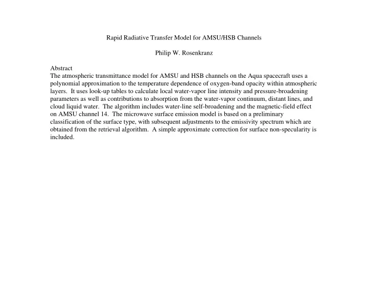
  1. Rapid Radiative Transfer Model for AMSU/HSB Channels Philip W. Rosenkranz Abstract The atmospheric transmittance model for AMSU and HSB channels on the Aqua spacecraft uses a polynomial approximation to the temperature dependence of oxygen-band opacity within atmospheric layers. It uses look-up tables to calculate local water-vapor line intensity and pressure-broadening parameters as well as contributions to absorption from the water-vapor continuum, distant lines, and cloud liquid water. The algorithm includes water-line self-broadening and the magnetic-field effect on AMSU channel 14. The microwave surface emission model is based on a preliminary classification of the surface type, with subsequent adjustments to the emissivity spectrum which are obtained from the retrieval algorithm. A simple approximate correction for surface non-specularity is included.
  2. 1. Atmospheric transmittance model a) For channels near a water line or in a window, at most one Lorentzian resonance factor is computed. Look-up tables are used to obtain the temperature dependence of: self and foreign continuum, self and foreign line broadening, line intensity, cloud-liquid absorption, fixed-gas opacity. b) Channels in the oxygen band use a third-order polynomial function of temperature to compute fixed-gas opacity. Channel 14 has a magnetic-field correction. Water-vapor and cloud-liquid opacity are computed as for a window channel.

  3. 2. Surface brightness model An a priori surface-brightness spectrum is chosen by a classification algorithm that operates on AMSU window channels. There are 7 classes: 0 Coastline 1 Land 2 Ocean 3 First-year sea ice or mixed ice/land/water 4 Multi-year sea ice or mixed ice/water 5 Snow over land 6 Glacier The mw retrieval algorithm subsequently adds a smooth 3-parameter correction curve to the a priori spectrum. Later stages of the retrieval can adjust the surface brightness curve uniformly (1 degree of freedom). ___________________________________________________________ 3. The radiative-transfer calculation uses an empirically determined correction factor of 1.15 for reflected-sky path length, to account for surface non-specularity.

  4. 4. Tests a. Comparison with line-by-line calculations Approximation errors are smaller than the instrument noise. b. Comparison of brightness temperature computed from radiosondes with NOAA-15 AMSU measurements Adjustments to data: Sidelobe corrections calculated by T. Mo Temperature profiles extended to 1 mb using retrieved profile, but the raob profile must extend to an altitude where transmittance to space = 0.9

  5. � 10 8 ch.5 6 53.6 GHz 4 2 obs−calc Tb, K 0 −2 −4 −6 −8 −10 −60 −40 −20 0 20 40 60 zenith angle, deg

  6. � 10 8 ch.7 6 54.94 GHz 4 2 obs−calc Tb, K 0 −2 −4 −6 −8 −10 −60 −40 −20 0 20 40 60 zenith angle, deg

  7. � 10 8 ch.9 57.29 GHz 6 4 2 obs−calc Tb, K 0 −2 −4 −6 −8 −10 −60 −40 −20 0 20 40 60 zenith angle, deg

  8. Table 1. Statistics of observed-minus-calculated differences in brightness temperature (all angles). The peak pressure is for the weighting function at vertical. The outlier threshold is 6K for channel 4, and 3K for the other channels. Channel 4 5 6 7 9 10 peak pressure (hPa) 1000 700 400 250 90 50 number of outliers 40 28 17 21 22 3 number of points used 1101 1040 979 894 673 324 mean (K) 0.19 0.23 -0.42 0.01 -0.36 -0.12 standard deviation (K) 1.54 0.64 0.55 0.63 0.73 0.74

  9. Error contributions: a) Radiometer noise b) Systematic measurement errors (calibration, sidelobe uncertainty) c) Radiosonde errors d) Sampling error (horizontal smoothing of temperature structure by antenna footprint) e) Forward-model errors Water-vapor channels to be validated with ARM raob launches. __________________________________________________ 5. Conclusions Forward algorithm is a faithful substitute for line-by-line transmittance calculation. Random differences with radiosonde calculations are largely accounted for by sources a, c, d, except for surface-sensitive channel. Systematic differences may be at least partly instrumental.

Download Presentation
Download Policy: The content available on the website is offered to you 'AS IS' for your personal information and use only. It cannot be commercialized, licensed, or distributed on other websites without prior consent from the author. To download a presentation, simply click this link. If you encounter any difficulties during the download process, it's possible that the publisher has removed the file from their server.

Recommend


More recommend