Ranked Query Processing: Relevance a) Order-based Paradigm - - PDF document

1

Ranked Query Processing: a) Order-based Paradigm

Kevin Chen-Chuan Chang

2

Ranking– Ordering according to the degree of some fuzzy notions:

Similarity (or dissimilarity) Relevance Preference

Q

ranking

3

Query models for order-based paradigm– On the better-than graph

Better-than graph Best-Matches-Only (BMO) query model

Retrieve maximal elements Thus also called maximal vector

These maximal elements form the “skyline”! On better-than graph, how to process BMO?

t4 t1 t2 t3

4

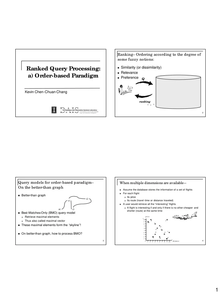
When multiple dimensions are available--

• Assume the database stores the information of a set of flights
• For each flight

Its price Its route (travel-time or distance traveled)

• A user would retrieve all the “interesting” flights

A flight is interesting if and only if there is no other cheaper and

shorter (route) at the same time

x y b a i k h g d f e c l

• 1

2 3 4 5 6 7 8 9 1 0 1 2 3 4 5 6 7 8 9 1 0

m n price distance

2

5

The overall preference combines the dimensions

P1 LOWEST(price)

a b i c, h g d, m f n k, e l

P2 LOWEST(distance)

k m, i h, n l f g d c a b, e

P :=({price,distance},<P1⊗P2) BMO: Maximal elements of P?

Is a maximal? Is b maximal? Is c maximal?

Distance Price a 1 9 b 2 10 c 4 8 d 6 7 e 9 10 f 7 5 g 5 6 h 4 3 i 3 2 k 9 1 l 10 4 m 6 2 n 8 3 6

Skyline Operation

Dominance: A point dominates another point if it is no worse in all

dimensions, and better in at least one dimension

Skyline: A set of all points in the dataset that are not

dominated by any other point in the dataset

7

Why is it called “skyline”?

(Also called: Pareto curve, Maximum Vector) What do you see in the Chicago skyline?

8

Query:

SELECT * FROM flights SKYLINE OF price MIN, distance MIN

What dominates what? What points constitute the skyline?

What is skyline: An example

x y b a i k h g d f e c l

• 1

2 3 4 5 6 7 8 9 1 0 1 2 3 4 5 6 7 8 9 1 0

m n price distance

3

9

Skyline Algorithms: We will look at a few examples

Block nested loop (BNL) Divide and Conquer Bitmap NN

10

Block Nested Loop [Börzsönyi et al., 2001]

Conceptually: Nested loop joins— Joining the table with itself Compare every pair of points to check dominance

Price Distance a 1 9 b 2 10 c 4 8 d 6 7 e 9 10 f 7 5 g 5 6 h 4 3 i 3 2 k 9 1 l 10 4 m 6 2 n 8 3 Price Distance a 1 9 b 2 10 c 4 8 d 6 7 e 9 10 f 7 5 g 5 6 h 4 3 i 3 2 k 9 1 l 10 4 m 6 2 n 8 3 11

Block Nested Loop -- Implementation

One-pass scan:

Scan the table; maintain a window of current skyline points Return the window at the end

Any problems?

Price Distance Skyline Discarded a 1 9 a b 2 10 a b c 4 8 a,c d 6 7 a,c,d e 9 10 a,c,d e f 7 5 a,c,d,f g 5 6 a,c,f, g d h 4 3 a, h c,f,g i 3 2 a, i h k 9 1 a,i,k l 10 4 a, i ,k l

Scan

12

Block Nested Look– Improvements How if the window overflow?

Multi-pass algorithm Scan the table, write any overflow to temp file Scan the temp file; repeat till done

Price Distance Skyline Discarded TempFile a 1 9 a b 2 10 a b c 4 8 a,c d 6 7 a,c,d e 9 10 a,c,d e f 7 5 a,c,d f g 5 6 a,c,g d h 4 3 a,h c,g i 3 2 a,i h k 9 1 a,i,k l 10 4 a, i ,k l

Scan Pass 1 Pass 2 Scan TempFile

4

13

Block Nested Look– Improvements How if the window overflow?

[Börzsönyi et al., 2001]

Divide and conquer

Divide all the points into several groups such that each group

fits in memory

Process the groups separately Merge their results

Smart merging possible

If s3 not empty then disregard s2 Use s3 to purge s1, s4

x y b a i k h g d f e c l

• 1

2 3 4 5 6 7 8 9 10 1 2 3 4 5 6 7 8 9 10

m n s1 s2 s3 s4 14

However, BNL-based approaches are not incremental– Want progressive processing!

Desired:

Compute the first few Skyline points almost instantaneously Compute more and more results incrementally

15

Bitmap Algorithm: Representation [Tan et. al.

2001]

For each dimension: n distinct values n bits A value as a bitmap of all no-higher bits = 1 4 3 2 1 3 2 1 2 1 a (1,1,2) 1 1 1 1 b (3,2,1) 1 1 1 1 1 1 c (4,1,1) 1 1 1 1 1 1 d (2,3,2) 1 1 1 1 1 1 1

d2: dist d3: rating d1: price

16

Is b = (3, 2, 1) in the skyline?

Any point with no-worse values in all dimensions?

0110 & 0101 & 1111 = 0100

Any point with a better value in some dimension?

0010 | 0001 | 1001 = 1011

Any point satisfying both?

0100 & 1011 = 0000

So, is b = (3,2,1) in the skyline?

d2: dist d3: rating d1: price

4 3 2 1 3 2 1 2 1 a (1,1,2) 1 1 1 1 b (3,2,1) 1 1 1 1 1 1 c (4,1,1) 1 1 1 1 1 1 d (2,3,2) 1 1 1 1 1 1 1

5

17

The Bitmap Algorithm

for each point x in DB: check if x is in skyline

• utput x if so

Incremental indeed; bitmap computation efficient However, any problem?

18

Bitmap Algorithm: Problems

Bitmaps are not dynamic structures Hard to update Bitmaps can have prohibitive space overhead How if there are many distinct values? E.g., How about continuous values? No focus of directions at all in skyline search Depend on what points you check first

19

NN – Finding the First Skyline Point [Kossmann et.

• al. 2002]
• Start by finding the nearest neighbor of the origin

I.e., the point p = (x, y) with the smallest How to find NN: Use NN algorithm based on R-tree.

This NN point must be in the skyline

Otherwise?

x y b a i k h g d f e c l

• 1

2 3 4 5 6 7 8 9 10 1 2 3 4 5 6 7 8 9 10

m n

2 2

) , ( y x p

• dist

+ =

20

NN– Are there other skyline points?

Pruning-- What cannot be in the skyline? Those dominated by point I Iteration– What may be in the skyline? Non-dominated region 2 and 3

x y b a i k h g d f e c l

• 1

2 3 4 5 6 7 8 9 10 1 2 3 4 5 6 7 8 9 10

m n

1 2 3 4

6

21

NN– Iteratively Process All the “ ToDo” Regions until All Done

x y b a i k h g d f e c l

• 1 2

3 4 5 6 7 8 9 10 1 2 3 4 5 6 7 8 9 10

m n

1 2 3 4

x y b a i k h g d f e c l

• 1

2 3 4 5 6 7 8 9 10 1 2 3 4 5 6 7 8 9 10

m n

1

3 4

2

x y b a i k h g d f e c l

• 1 2

3 4 5 6 7 8 9 10 1 2 3 4 5 6 7 8 9 10

m n

1

3

2 4

i a k

22

Order-based rank query evaluation-- Still

• ngoing research.

How optimal are these algorithms? Further

improvement?

Scale to high dimensionality? Generalize to non-BMO type of aggregations?

23

Thank You!

Ranking Query Processing: b) Score-based Paradigms

Kevin Chen-Chuan Chang

7

25

Ranking– Ordering according to the degree of some fuzzy notions:

Similarity (or dissimilarity) Relevance Preference

Q

ranking

26

Relational DBMS scenarios– A brief overview Relational DBMS–

Value mapping: [Chaudhuri and Gravano, 1999] Mapping top-k scores to Boolean selection ranges May have to restart Cardinality mapping: [Carey and Kossmann, 1997, 1998] Pushing “limit k” down query tree May have to restart

27

Our Focus: Middleware scenarios

Top -k Algorithm F=min(p1, p2, p3)

k=10

p1 p3 top results

select h.id, h.addressfrom Hotel h

• rder by F=min(

p1:rating(h.rate), p2:cheap(h.price), p3:safe(h.zip)) stop after k=10

p2 RDBMS hotels.com apbs.com

28

Top-k algorithms rely on accesses to evaluate query scores

To each predicate pi:

• Random access:ra

i(uj)

• Return score of uj for pi
• Sorted access: sa

i

• Return some next best object and

its score for p i

p1 uj p1[uj]

u3: .70 u2: .65 u1: .60

p1

8

29

Sorted access on P1 then random accesses to P2, P2

An algorithm performs a sequence of accesses: A simple algorithm

Sort

p1 p3 top result p2 RDBMS hotels.com apbs.com

c:.80 b:.45 a:.30 a:.8 b:.90 c:.90 a:.9 b:.70 c:.95 c:.80 F=min(p1, p2, p3)

k=1

30

Goal: Minimize the “ access” cost

Access costs dominate in “middleware” scenarios Cost model: aggregate of all access costs RDBMS cheap safe rating

Top -k Algorithm F, k

hotels.com apbs.com

s2=44ms, r

2=466ms

s3=∞, r3=700ms s1=3ms, r1=20ms

31

Assumption: Monotonic scoring functions

Monotonic:

f(x1, …, xn) ≤ f(x1′, …, x n′) if xi ≤ xi′ for all i

Why good for query evaluation?

Gives bounds for pruning data Gives a simple function “surface” to maximize f

Reasonable?

Analogy: Negation rarely used in Boolean queries But, new “function-inference” front -ends also found this to be

violated in many cases

32

The Naïve Algorithm

Get all pi[u] score for every object u e.g., by complete sorted accesses Compute F[u] = F (p1[u],…, pm [u] ) for every u Sort Return top

k

Obviously expensive. Can we do better? Note k is typically small

9

33

FA– Fagin’s Algorithm (or the “First Algorithm”) [Fagin,

1996] [Wimmerset al., 1999]

Scenario: Sorted + Random Access Available

Go in the lists with SA in parallel Do complete RA for every seen object to complete scores Maintain a buffer of current top-k objects Maintain a threshold T:

Upper-bound for all the unseen objects

Stop:

When all lists so far share at least k objects

Return the current top-k objects

34

FA– Fagin’s Algorithm

Scoring function: F= p1+p2 ID 3 2 1 4 5

p2

.50 .40 .30 .20 .10

p1

.50 .40 .30 .20 .10 ID 5 1 3 2 4 Buffer 3: (.80) 5: (.60) 3: (.80) 1: (.70) 5: (.60) 2: (.60)

Intersection {} {} {1, 3}

35

Why is FA correct?

At stop time, all seen objects are compared Can unseen objects have higher scores? e.g., How about object 4? Upper bound? ID 3 2 1 4 5

p2

.50 .40 .30 .20 .10

p1

.50 .40 .30 .20 .10 ID 5 1 3 2 4

Intersection {} {} {1, 3}

Buffer 3: (.80) 1: (.70) 5: (.60) 2: (.60) 36

How is FA “optimal”? Can you make it more efficient?

FA: For string, monotone F, sorted accesses optimal up

to a constant factor, with high probability.

Can you stop earlier than round 3? ID 3 2 1 4 5

p2

.50 .40 .30 .20 .10

p1

.50 .40 .30 .20 .10 ID 5 1 3 2 4

Intersection {} {} {1, 3}

Buffer 3: (.80) 1: (.70) 5: (.60) 2: (.60)

10

37

Then, there have been various algorithms, for different scenarios...

FA, TA, QuickCombine r =1 (cheap) r = h (expensive) r = ∞ (impossible) CA, SR-Combine NRA, StreamCombine TAz, MPro, Upper s =1 (cheap) s = h (expensive) s = ∞ (impossible)

Random Access Sorted Access

FA, TA, QuickCombine TAz, MPro, Upper NRA, StreamCombine

38

Improving FA: TA [Fagin et al., 2001], Quick-combine

[Guentzer et al., 2000], Multi-step [Nepal and Ramakrishna, 1999]

Scenario: Sorted + Random Access Available

Go in the lists with SA in parallel Do complete RA for every seen object to complete scores Maintain a buffer of current top-k objects Maintain a threshold T:

Upper-bound for all the unseen objects

Stop:

When all current top-k objects scored greater than T

Return these objects as top-k

39 T = 1.00

TA, Quick-combine, Multi-step F= p1 + p2

ID 3 2 1 4 5 S2 .50 .40 .30 .20 .10 S1 .50 .40 .30 .20 .10 ID 5 1 3 2 4 Buffer 3: (.80) 1: (.70) 5: (.60) 2: (.60) T = .80

Threshold

3: (.80) 5: (.60) 40

Why is TA correct?

At stop time, all seen objects are compared Can unseen objects have higher scores? e.g., How about object 4? Upper bound? T = 1.00 ID 3 2 1 4 5 S2 .50 .40 .30 .20 .10 S1 .50 .40 .30 .20 .10 ID 5 1 3 2 4 Buffer 3: (.80) 1: (.70) 5: (.60) 2: (.60) T = .80

Threshold

3: (.80) 5: (.60)

11

41

Observations: Any Problem with TA?

How does it handle SA? Equal-depth parallel SA to every list How does it handle RA? Exhaustive RA for every seen object How if RA expensive? (Algorithm CA) How if RA not possible? (Algorithm NRA)

42

How if random accesses not supported?

The combined score of an object has two parts:

Upper bound score:

From seen exact scores and unseen max score

Lower bound score:

From seen exact scores and unseen min score

An object is in top-k if

Its lower bound score is greater than the upper bound

scores of all unseen objects

43

NRA [Fagin etal., 2001], Stream-combine [Guentzer et al., 2001] -- When random accesses not possible

Scoring function: F= p1 + p2 ID 3 2 1 4 5 S2 .50 .40 .30 .20 .10 S1 .50 .40 .30 .20 .10 ID 5 1 3 2 4 Buffer 5: (.50 – 1.00) 3: (.50 – 1.00) 5: (.50 – .90) 3: (.50 – .90) 1: (.40 – .80) 2: (.40 – .80) 3: (.80 – .80) 1: (.70 – .70) 5: (.50 – .80) 2: (.40 – .70)

44

In contrast, how if sorted accesses not possible? Scenario: When SA not supported

Perform random “probes” when necessary The object with current highest score Schedule predicates to minimize probes Return an object as top-k when It is fully probed Its score is higher than the (upper bounds of) the

rest not in top-k

12

45

MPro [Chang and Hwang, 2002], Upper [Bruno et. al. 2002] – When sorted accesses not possible

.75 .78 .20 .60 .50 .75 .90 .20 .90 .80 .85 .78 .75 .90 .70 0.90 0.80 0.70 0.60 0.50 a b c d e

Min(x,p1,p2 )

p2 p1 x ID

a: 0.9 a: 0.85

Uunseen=

a: 0.85 b: 0.8 b: 0.8 a: 0.75 b: 0.78 a: 0.75 0.7 b: 0.78 a: 0.75 c: 0.7 b: 0.78 a: 0.75 c: 0.7 Candidates Queue

Upper-bound of the unseen scores

46

Probe optimization– Is the cost of random probes minimal?

What object to probe next?

By necessary probes to analytically determine

[Chang and Hwang, 2002]

• Current top object must be further probed (by any algorithm)

For such object, what predicate to probe next?

MPro: Global scheduling – one schedule for all

• Cost- based optimization based on selectivity and cost

Upper: Local scheduling – schedule for each obj

• Use expected scores of unknown objects

47

So, what do we have so far…

FA, TA, QuickCombine r =1 (cheap) r = h (expensive) r = ∞ (impossible) CA, SR-Combine NRA, StreamCombine TAz, MPro, Upper s =1 (cheap) s = h (expensive) s = ∞ (impossible)

Random Access Sorted Access

FA, TA, QuickCombine TAz, MPro, Upper NRA, StreamCombine

What do you think?

48

Challenge: Various Cost Scenarios

Vary in capabilities Vary in costs:

• ver sources
• ver access types
• ver time

Thus requires “ generality” over cost scenarios

and “ adaptivity” to the given runtime setting

RDBMS cheap safe rating

Top -k Algorithm

hotels.com apbs.com

s2=44ms, r

2=466ms

s3=∞, r3=700ms s1=3ms, r1=20ms

13

49

Score-based ranked query evaluation– Still

• ngoing research

A unified algorithms for all? Currently: ad-hoc algorithms for each scenario Do not cover all scenarios How optimal are these algorithms? Cost-based optimization studied at MPro Unified, cost-based optimization?

50

Thank You!