Quiz Let q 1 , . . . , q n be orthonormal vectors in R m . Let V = - PowerPoint PPT Presentation

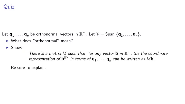
Quiz Let q 1 , . . . , q n be orthonormal vectors in R m . Let V = Span { q 1 , . . . , q n } . ◮ What does “orthonormal” mean? ◮ Show: There is a matrix M such that, for any vector b in R m , the the coordinate representation of b ||V in terms of q 1 , . . . , q n can be written as M b . Be sure to explain.

Projection onto columns of a column-orthogonal matrix Suppose q 1 , . . . , q n are orthonormal vectors. � q j , b � Projection of b onto q j is b || q j = σ j q j where σ j = � q j , b � � q j , q j � = Vector [ σ 1 , . . . , σ n ] can be written using dot-product definition of matrix-vector multiplication:   q T    q 1 · b    σ 1 1   . . .   . . .  =  = b       . . .         q T q n · b σ n   n       σ 1     .   . and linear combination σ 1 q 1 + · · · + σ n q n = q 1 · · · q n   .       σ n      

Towards QR factorization Orthogonalization of columns of matrix A gives us a representation of A as product of ◮ matrix with mutually orthogonal columns ◮ invertible triangular matrix      1  α 12 α 13 α 1 n 1 α 23 α 2 n             1 α 3 n          v ∗ v ∗ v ∗ v ∗  v 1 v 2 v 3 · · · v n = · · ·  ...     n  1 2 3               α n − 1 , n           1 Suppose columns v 1 , . . . , v n are linearly independent. Then v ∗ 1 , . . . , v ∗ n are nonzero. ◮ Normalize v ∗ 1 , . . . , v ∗ n (Matrix is called Q ) ◮ To compensate, scale the rows of the triangular matrix. (Matrix is R ) The result is the QR factorization. Q is a column-orthogonal matrix and R is an upper-triangular matrix.

Towards QR factorization Orthogonalization of columns of matrix A gives us a representation of A as product of ◮ matrix with mutually orthogonal columns ◮ invertible triangular matrix � v ∗  1 �  β 12 β 13 β 1 n    � v ∗ 2 � β 23 β 2 n       � v ∗  3 � β 3 n          ...     v 1 v 2 v 3 v n q 1 q 2 q 3 q n · · · = · · ·                       β n − 1 , n      � v ∗ n � Suppose columns v 1 , . . . , v n are linearly independent. Then v ∗ 1 , . . . , v ∗ n are nonzero. ◮ Normalize v ∗ 1 , . . . , v ∗ n (Matrix is called Q ) ◮ To compensate, scale the rows of the triangular matrix. (Matrix is R ) The result is the QR factorization. Q is a column-orthogonal matrix and R is an upper-triangular matrix.

Using the QR factorization to solve a matrix equation A x = b First suppose A is square and its columns are linearly independent. Then A is invertible. It follows that there is a solution (because we can write x = A − 1 b ) QR Solver Algorithm to find the solution in this case: Find Q , R such that A = QR and Q is column-orthogonal and R is triangular Compute vector c = Q T b Solve R x = c using backward substitution, and return the solution. Why is this correct? ◮ Let ˆ x be the solution returned by the algorithm. ◮ We have R ˆ x = Q T b ◮ Multiply both sides by Q : Q ( R ˆ x ) = Q ( Q T b ) ◮ Use associativity: ( QR )ˆ x = ( QQ T ) b ◮ Substitute A for QR : A ˆ x = ( QQ T ) b ◮ Since Q and Q T are inverses, we know QQ T is identity matrix: A ˆ x = 1 b Thus A ˆ x = b .

Solving A x = b What if columns of A are not independent? Let v 1 , v 2 , v 3 , v 4 be columns of A . Suppose v 1 , v 2 , v 3 , v 4 are linearly dependent. Then there is a basis consisting of a subset, say v 1 , v 2 , v 4     x 1       x 2    v 1   v 2 v 3 v 4  : x 1 , x 2 , x 3 , x 4 ∈ R =    x 3       x 4        x 1    v 1  : x 1 , x 2 , x 4 ∈ R v 2 v 4 x 2   x 4   Therefore: if there is a solution to A x = b then there is a solution to A ′ x ′ = b where columns of A ′ are a subset basis of columns of A (and x ′ consists of corresponding variables). So solve A ′ x ′ = b instead.

The least squares problem Suppose A is an m × n matrix and its columns are linearly independent.   x 1 Since each column is an m -vector, dimension of   1 2 3 4 5 x 2   column space is at most m , so n ≤ m .   6 7 8 9 10 = b x 3       11 12 13 14 15 x 4 What if n < m ? How can we solve the matrix   x 5 equation A x = b ? Remark: There might not be a solution:   1 2 3   x 1 ◮ Define f : R n − → R m by f ( x ) = A x 4 5 6  = b   x 2    7 8 9 ◮ Dimension of Im f is n   x 3 10 11 12 ◮ Dimension of co-domain is m . ◮ Thus f is not onto. Goal: An algorithm that, given a matrix A whose columns are linearly independent and given b , finds the vector ˆ x minimizing � b − A ˆ x � . Solution: Same algorithm as we used for square A

The least squares problem Recall... High-Dimensional Fire Engine Lemma: The point in a vector space V closest to b is b ||V and the distance is � b ⊥V � . Given equation A x = b , let V be the column space of A . x = b ||V . We need to show that the QR Solver Algorithm returns a vector ˆ x such that A ˆ

Projection onto columns of a column-orthogonal matrix Suppose q 1 , . . . , q n are orthonormal vectors. � q j , b � Projection of b onto q j is b || q j = σ j q j where σ j = � q j , b � � q j , q j � = Vector [ σ 1 , . . . , σ n ] can be written using dot-product definition of matrix-vector multiplication:   q T    q 1 · b    σ 1 1   . . .   . . .  =  = b       . . .         q T q n · b σ n   n       σ 1     .   . and linear combination σ 1 q 1 + · · · + σ n q n = q 1 · · · q n   .       σ n      

QR Solver Algorithm for A x ≈ b Summary: ◮ QQ T b = b || Proposed algorithm: Find Q , R such that A = QR and Q is column-orthogonal and R is triangular Compute vector c = Q T b Solve R x = c using backward substitution, and return the solution ˆ x . Goal: To show that the solution ˆ x returned is the vector that minimizes � b − A ˆ x � Every vector of the form A x is in Col A (= Col Q ) By the High-Dimensional Fire Engine Lemma, the vector in Col A closest to b is b || , the projection of b onto Col A . Solution ˆ x satisfies R ˆ x = Q T b x = QQ T b Multiply by Q : QR ˆ x = b || . Therefore A ˆ

Least squares when columns are linearly de pendent? This comes up, e.g. ranking sports teams. Need a more sophisticated algorithm. We’ll see it soon.

The Normal Equations Let A be a matrix with linearly independent columns. Let QR be its QR factorization. We have given one algorithm for solving the least-squares problem A x ≈ b : Find Q , R such that A = QR and Q is column-orthogonal and R is triangular Compute vector c = Q T b Solve R x = c using backward substitution, and return the solution ˆ x . However, there are other ways to find solution. Not hard to show that ◮ A T A is an invertible matrix ◮ The solution to the matrix-vector equation ( A T A ) x = A T b is the solution to the least-squares problem A x ≈ b ◮ Can use another method (e.g. Gaussian elimination) to solve ( A T ) x = A T b The linear equations making up A T A x = A T b are called the normal equations.

Application of least squares: linear regression Finding the line that best fits some two-dimensional data. Data on age versus brain Let f ( x ) be the function that predicts brain mass for someone of age mass from the Bureau of x . Made-up Numbers: Hypothesis: after age 45, brain mass decreases linearly with age, i.e. that f ( x ) = mx + b for some numbers m , b . age brain mass Goal: find m , b to as to minimize the sum of squares of prediction 45 4 lbs. errors 55 3.8 The observations are ( x 1 , y 1 ) = (45 , 4), ( x 2 , y 2 ) = (55 , 3 . 8), 65 3.75 ( x 3 , y 3 ) = (65 , 3 . 75),( x 4 , y 4 ) = (75 , 3 . 5), ( x 5 , y 5 ) = (85 , 3 . 3). 75 3.5 The prediction error on the i th observation is | f ( x i ) − y i | . 85 3.3 i ( f ( x i ) − y i ) 2 . The sum of squares of prediction errors is � For each observation, measure the difference between the predicted and observed y -value. In this application, this difference is measured in pounds. Measuring the distance from the point to the line wouldn’t make sense.