SLIDE 1 QUANTUM INTERFERENCE & QUANTUM PATHS
PCES 12.1
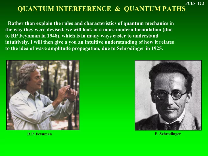
Rather than explain the rules and characteristics of quantum mechanics in the way they were devised, we will look at a more modern formulation (due to RP Feynman in 1948), which is in many ways easier to understand
- intuitively. I will then give a you an intuitive understanding of how it relates
to the idea of wave amplitude propagation, due to Schrodinger in 1925.
R.P. Feynman
SLIDE 2 PCES 12.2
There is NO WAY to understand the passage of quantum particles via 2 slits as ‘particles’- they show wavelike interference. On the other hand we cannot understand their propagation as mere waves either- they arrive in “lumps”.
Classical probabilities for the passage of classical particles through 1 or 2 slits
Let us recall again the mysterious feature
- f quantum mechanics that began to be
uncovered in the work of Newton and Huyghens:
Particle – Wave DUALITY DUALITY
Wave interference between 2 sources Probabilities for passage of quantum particles via slits
SLIDE 3 PCES 12.3
The QUANTUM RULES - Sum over PATHS
Now we come to the strange rules of quantum mechanics. Here I am going to tell you the version of them that was invented by Feynman in 1948. It goes as follows: (1) First we find a quantity called the QUANTUM AMPLITUDE for a system to go from one quantum state ψ1 to another state ψ2 . This amplitude we call G21 . (2) Now, to find out what the amplitude is we imagine that the system simultaneously tries to go over ALL POSSIBLE PATHS between the 2
- states. We give each path a weight, as though a wave was propagating
along this path. Then, we add up all the weights- AS THOUGH THE SYSTEM REALLY WAS TRAVELLING OVER ALL THE PATHS AT THE SAME TIME. Then the PROBABILITY that the system goes from the first to the second state is just P21 = |G21|2
Feynman (1920-87)
SLIDE 4
PCES 12.4 Small deviations about a path
PROPERTIES of QUANTUM PATHS
Since any path is allowed, most paths are tortuous. However most interfere destructively because they all have different phases (different total number of waves) between start & finish. However CLASSICAL PATHS hardly change phase with small change in path- all these paths then interfere constructively. The paths of large classical objects are ones where the phase is a maximum or minimum (hardly varying with slight changes). In many quantum systems the paths involve different particles, interacting with each other. If we look closely at any interaction, we see a “sub-structure” of more complex interaction paths. This small-scale structure involves high- momentum (& hence high-energy) Processes (recall de Broglie’s relation p = h/λ which says short wavelengths have high momentum)
The real complexity of the path Magnifying up the path in a process (here electron- electron scattering) Electron-photon scattering
SLIDE 5 PCES 12.5
QUANTUM PATHS: Plane Waves
The simplest kind of motion involves plane waves, traveling in some direction- corresponding classically (in the limit of short wavelength) to a particle moving in a straight line with p = h/λ. If the plane wave interacts with some small localised object, part of it will continue on but part will be scattered- ie., re-emitted as a wave propagating away from the
- bject. This is roughly what happens in Rutherford scattering off the nucleus.
Left: plane wave states with 2 different momenta (& so different wavelengths). Above: lane wave scatters
QUANTUM PATHS: Multiple Slits
One way to look in more detail at the way that different paths interfere is to have multiple slit set-ups. In this way one is giving the quantum system a “multiple-choice” set of paths to follow- but restricted by having to pass through the slits. One can then verify that (i) the final quantum amplitude to get to a point on the screen is indeed found by summing over all intermediate paths; & (ii) that the amplitude re-radiates from each slit a la Huyghens.
Propagation through multiple slits
SLIDE 6 PCES 12.6
One fascinating effect which is impossible to understand classically is shown nicely by a set-up in which electrons go around 2 paths (allowing interference between the paths), with a region of non-zero magnetic field inside the loop. The field never touches the loop- the electrons move in a field-free region (most easily arranged with a superconducting ring). The Aharonov-Bohm prediction (1959) was that changing the field inside the ring would change the interference pattern- even though the fields were always zero along the electron paths! Even far from the field, the wave- function senses the change.
A 2-slit experiment for electrons, Passing via a superconducting
Left: the experimental results- the current shows 2-slit interference, which can be changed by varying the field.
Non-local Interference- the Aharonov-Bohm effect
SLIDE 7 PCES 12.7
“Bound States” of Quantum Systems
As we saw with the discussion of Schrodinger’s formulation of Q.M., confining a quantum system means the wave amplitudes can’t propagate freely- instead they form “standing waves” (sums of waves and their reflections) inside the confining region- called “eigenstates” The lowest-energy bound state is called the “ground state”- the higher energy states, with shorter wavelengths, are called “excited states”. We go from one energy level to the next highest one by fitting in one more oscillation.
Energy levels and wave-functions in a
the no. of oscillations
As we already saw with the H atom, the existence of discrete energy levels means that the bound system can
- nly change its energy by certain amounts (the quantum
jumps), unless the system is excited by some external energy source all the way out of the potential well. If this happens (for an atom we would say it is “ionized”) then a continuum of free states is available- the particle escapes.
Wave-functions for bound states inside the potential well shown at the top.
SLIDE 8
“SPIN” in QUANTUM MECHANICS
We have seen that a quantum particle moves through space as a “probability wave”. And de Broglie saw that rotational angular motion of an object is also described by a probability wave- the waves correspond to different discrete values of angular momentum (ie., the rotational velocity of a quantum system is also quantized). A startling feature of quantum mechanics is that even a point particle has a property called SPIN. Actually there are 2 classes of particle in Nature. Those called FERMIONS can only have “half integer” spin- the simplest are spin-1/2 particles, but one also has particles with spin 3/2, 5/2, etc. Then there are BOSONS, with “integer” spin, ie., spin 1, or 2,3, etc. The angular momentum of a spin s is hs, where h is again Planck’s constant. What is also quantized is the value of the spin along any direction. A spin-1/2 then has spin either ‘up’ (ie., 1/2) or ‘down’ (ie., -1/2) along a vertical z-axis. But if we measure an up spin along the x- axis, we find not zero, but ‘left’ or ‘right’ with equal (50%) probability- the up spin is a quantum sum (or ‘superposition’) of the left & right states. At left we see the Stern-Gerlach apparatus, in which a beam of spin-1/2 particles is separated according to their spin along the z- axis.
Randomly-oriented classical spins separated according to the Z-component of their spin Same for spin-1/2 quantum spins- only 2 values allowed. PCES 12.8
SLIDE 9 The electrons fill up the different states in the -Z/r potential around the nucleus, where Z is the + charge of the nucleus (equal to the number of protons in the nucleus). The H atom, with a radius ~ 10-10 m, and a single proton nucleus with 1 electron around it, is the simplest. The electron states are labelled by the number n of radial oscillations, but also by oscillations as one moves around the nucleus (telling us the angular momentum). The bound states are at the Bohr energies
εn = -R/n2
below the continuum states, where R ~ 13.6 eV (electron Volts).
Artist impression of some atoms probablities for 2 different electron states in H. Top: allowed transitions between the different levels in a H atom- the levels have the Bohr
probability for the electron in some states to be at a distance r from the nucleus PCES 12.9
ATOMIC STRUCTURE
SLIDE 10
PCES 12.10
QUANTUM TUNNELING
Tunneling through a barrier.
Another interesting property of waves is that they “leak” through classically “forbidden” zones- for quantum waves this is called “quantum tunneling”. In the high-energy forbidden regions the waves decay, so penetration only happens if the barrier is thin. The effect of tunneling is that what were formerly stable systems (either confined by potential barriers, or by short-range attractive forces), now can decay in some way. Such tunneling transitions are crucial in Q.M.; they allow communication between states that cannot communicate classically.
The attractive potential energy well preventing nuclear fission
The first example of tunneling was discussed in 1927; it is the process by which parts of a nucleus break away from strong attractive forces- ie., radioactive decay (right).