QUANDLE COCYCLES FROM GROUP COCYCLES YUICHI KABAYA Abstract. We give - - PDF document

QUANDLE COCYCLES FROM GROUP COCYCLES

YUICHI KABAYA

• Abstract. We give a construction of a quandle cocycle from a group cocycle, especially

an explicit construction of quandle cocycles of the dihedral quandle Rp from group cocy- cles of the cyclic group Z/p. The 3-dimensional group cocycle of Z/p gives a non-trivial quandle 3-cocycle of Rp.

• 1. Introduction

A quandle, which was introduced by Joyce [Joy], is an algebraic object whose axioms are motivated by knot theory and conjugation in a group. In [CJKLS], the authors introduced a quandle homology theory, and they defined the quandle cocycle invariants for classical knots and surface knots. The quandle homology is defined as the homology of the chain complex generated by cubes whose edges are labeled by elements of a quandle. On the other hand the group homology is defined as the homology of the chain complex generated by tetrahedra whose edges are labeled by elements of a group. So it is natural to ask a relation between quandle homology and group homology. In [IK], the authors defined a simplicial version of quandle homology and constructed a homomorphism from the usual quandle homology to the simplicial quandle homology. Applying the construction for PSL(2, C)-representation of the knot complement, we ob- tained a diagrammatic formula of the hyperbolic volume and the Chern-Simons invariant. The important point of [IK] is to give a triangulation of a knot complement in alge- braic fashion by using quandle homology. This construction enable us relate the quandle homology with the topology of a knot complement. In this note, we apply the work [IK] for finite quandles to construct quandle cocycles from group cocycles. Especially we construct quandle cocycles of the dihedral quandle Rp from group cocycles of the cyclic group Z/p. It will be shown that the 3-dimensional group cocycle gives a non-trivial quandle 3-cocycle of H3

Q(Rp; Z/p). Since dim H3 Q(Rp; Z/p) = 1,

• ur quandle 3-cocycle is a constant multiple of the Mochizuki’s 3-cocycle [Moc].

This note is organized as follows. We will review the definition of quandles and their homology theory in Section 2. In Section 3, we recall the definition of the group homology. We will review the construction of [IK] in Section 5 and apply it to construct quandle cocycles of a dihedral quandle. We will propose a general construction in Section 7.

• 2. Quandle and Quandle homology

A quandle is a set X with a binary operation ∗ satisfying the following axioms: (1) x ∗ x = x for any x ∈ X, (2) the map ∗y : X → X defined by x → x ∗ y is a bijection for any y ∈ X, (3) (x ∗ y) ∗ z = (x ∗ z) ∗ (y ∗ z) for any x, y, z ∈ X.

1

y g x z z y g(x, y, z) ((x ∗ y) ∗ z) x ∗ z z z x ∗ y y ∗ z y ∗ z gz gy g z x ∗ y x ∗ z y y y ∗ z ((x ∗ y) ∗ z) z x x y z z g gx g

Figure 1. ∂(g(x, y, z)) = −(g(y, z) − gx(y, z)) + (g(x, z) − gy(x ∗ y, z)) − (g(x, y) − gz(x ∗ z, y ∗ z)). Here x, y, z ∈ X and g ∈ GX. Edges are labeled by elements of X and vertices are labeled by elements of GX. We denote the inverse of ∗y by ∗−1y. For a quandle X, we define the associated group GX by x ∈ X|y−1xy = x ∗ y (x, y ∈ X). A quandle X has a right GX-action in the following way. Let g = xε1

1 xε2 2 · · · xεn n be an element of GX where xi ∈ X and εi = ±1.

Define x ∗ g = (· · · ((x ∗ε1 x1) ∗ε2 x2) · · · ) ∗εn xn. One can easily check that this is a right action of GX on X. So the free abelian group Z[X] generated by X is a right Z[GX]-module. Let CR

n (X) be the free (left) Z[GX]-module generated by Xn. We define the boundary

map CR

n (X) → CR n−1(X) by

∂(x1, x2, . . . , xn) =

n

∑

i=1

(−1)i((x1, . . . , xi, . . . , xn) − xi(x1 ∗ xi, . . . , xi−1 ∗ xi, xi+1, . . . , xn)). Figure 1 shows a graphical picture of the boundary map. Let CD

n (X) be the Z[GX]-

submodule of CR

n (X) generated by (x1, . . . , xn) with xi = xi+1 for some i. Now CD n (X)

is a subcomplex of CR

n (X). Let CQ n (X) = CR n (X)/CD n (X). For a right Z[GX]-module M,

we define the rack homology of M by the homology of CR

n (X; M) = M ⊗Z[GX] CR n (X) and

denote it by HR

n (X; M). We also define the quandle homology of M by the homology of

M ⊗Z[GX] CQ

n (X) and denote it by HQ n (X; M). The homology HQ n (X; Z), here Z is the

trivial Z[GX]-module, is equal to the usual quandle homology HQ

n (X). Let Y be a set

with a right GX-action. For any abelian group A, the abelian group A[Y ] generated by Y over A is a right Z[GX]-module. The homology group HQ

n (X; A[Y ]) is usually denoted

by HQ

n (X; A)Y ([Kam]).

Let N be a left Z[GX]-module. We define the rack cohomology Hn

Q(X; N) by the

cohomology of Cn

R(X; N) = HomZ[GX](CR n (X), N). The quandle cohomology Hn Q(X; N)

is defined in a similar way. For a set Y with a right GX-action and an abelian group A, we let Func(Y, A) be the left Z[GX]-module generated by functions φ : Y → A, here the action is defined by (gφ)(y) = φ(yg) for y ∈ Y and g ∈ GX. The cohomology group Hn

Q(X; Func(Y, A)) is usually denoted by Hn Q(X; A)Y .

2

• 3. Group homology

3.1. Let G be a group. Let Cn(G) be the free Z[G]-module generated by [g1| . . . |gn] ∈ Gn. Define the boundary map ∂ : Cn(G) → Cn−1(G) by ∂([g1| . . . |gn]) = g1[g2| . . . |gn] +

n−1

∑

i=1

(−1)i[g1| . . . |gigi+1| . . . |gn] + (−1)n[g1| . . . |gn−1]. Let C0(G) ∼ = Z[G] → Z → 0 be the augmentation map. We remark that the chain complex {· · · → C1(G) → C0(G) → Z → 0} is acyclic. So the chain complex C∗(G) gives a free resolution of Z. Let M be a right Z[G]-module. The homology of M ⊗Z[G] Cn(G) is called the group homology of M and denoted by Hn(G; M). In other words, Hn(G; M) = TorZ[G]

n

(M, Z). Let C′

n(G) be the free Z-module generated by (g0, . . . , gn) ∈ Gn+1. Then C′ n(G) is a left

Z[G]-module by g(g0, . . . , gn) = (gg0, . . . , ggn). Define the boundary operator of C′

n(G)

by ∂(g0, . . . , gn) =

n

∑

i=0

(−1)i(g0, . . . , gi, . . . , gn). C∗(G) and C′

∗(G) are isomorphic as chain complexes. In fact, the following correspondence

gives an isomorphism: [g1|g2| . . . |gn] ↔ (1, g1, g1g2, . . . , g1 · · · gn) ( g0[g−1

0 g1|g−1 1 g2| . . . |g−1 n−1gn] ↔ (g0, . . . , gn)

) The notation using (g0, . . . , gn) is called homogeneous and the one using [g1| . . . |gn] is called inhomogeneous. Factoring out Cn(G) by the degenerate complex, that is generated by [g1| . . . |gn] with gi = 1 for some i, we obtain the normalized chain complex and its homology group. It is known that the group homology using the normalized chain complex coincides with the unnormalized one. In homogeneous notation, we factor out C′

n(G) by the subcomplex

generated by (g0, . . . , gn) with gi = gi+1 for some i. 3.2. Let X be a quandle and M be a right Z[GX]-module. We can construct a map from the rack homology HR

n (X; M) to the group homology Hn(GX; M). The following lemma

is well-known. Lemma 3.1. Let · · · → P1 → P0 → M → 0 be a chain complex where Pi are projective (e.g. free). Let · · · → C1 → C0 → N → 0 be an acyclic complex. Any homomorphism M → N can be extended to a chain map from {P∗} to {C∗}. Moreover such a chain map is unique up to chain homotopy. So there exists a unique chain map from CR

∗ (X) to C∗(GX) up to homotopy. This map

induces M ⊗Z[GX] CR

∗ (X) → M ⊗Z[GX] C∗(GX) and then HR n (X; M) → Hn(GX; M). We

can also construct a natural map HQ

n (X; M) → Hn(GX; M). We give an explicit chain

• map. Let (x1, . . . , xn) be a generator of CR

n (X). We define the map f by

f((x1, . . . , xn)) = ∑

σ∈Sn

sgn(σ)[yσ,1| · · · |yσ,i| · · · |yσ,n]

3

x ∗ y x z z z z y y (x ∗ y) ∗ z x ∗ z y ∗ z y ∗ z

Figure 2 where yσ,i ∈ X is defined for a permutation σ and i ∈ {1, . . . , n} as follows. Let j1, . . . , ji < i be the maximal set of numbers satisfying σ(i) < σ(j1) < σ(j2) < · · · < σ(ji). Then define yσ,i = xσ(i) ∗ (xσ(j1)xσ(j2) · · · xσ(ji)). The graphical picture of this map is given in Figure 2. Example 3.2. Let (x, y, z) ∈ CR

3 (X).

Then the chain map f : CR

3 (X) → C3(GX)

constructed above is given by ∂((x, y, z)) =[x|y|z] − [x|z|y ∗ z] + [y|z|(x ∗ y) ∗ z] − [y|x ∗ y|z] + [z|x ∗ z|y ∗ z] − [z|y ∗ z|(x ∗ y) ∗ z]. If we use the normalized chain complex for group homology, we obtain a map f : CQ

3 (X) →

C3(GX). Remark 3.3. Fenn, Rourke and Sanderson defined the rack space BX. Since π1(BX) is isomorphic to GX, there exists a unique map, up to homotopy, from BX to the Eilenberg-MacLane space K(GX, 1) which induces the isomorphism between their fun- damental groups. The map we have constructed is essentially same as this map. As we have seen, there exists a relation between quandle homology and group homology. We shall give another relation which seems to reflect more geometric feature.

• 4. Shadow coloring and the cycle invariant

The contents of this section will be used in Section 7.3. 4.1. Let X be a quandle. Let K be an oriented knot in S3 and D be a diagram of K. An arc coloring is a map A : {arcs of D} → X if it satisfies the relation

x ∗ y y x

at each crossing, where x, y ∈ X. By the Wirtinger presentation of a knot complement, an arc coloring determines a representation π1(S3 \ K) → GX. This is obtained by sending each meridian to its color.

4

Let Y be a set with a right GX action. A map D : {regions of D} → Y is called a region coloring if it satisfies the relation

x r r · x

for any pair of adjacent regions, where r ∈ Y and x ∈ X. A pair S = (A, R) is called a shadow coloring. We define a cycle [C(S)] of HQ

2 (X; Z[Y ]) for a shadow coloring S. Assign +r ⊗ (x, y)

for a positive crossing colored by

r x y

and −r ⊗(x, y) for a negative crossing colored by

r x y

. Then define C(S) = ∑

c:crossing

εcrc ⊗ (xc, yc) ∈ CQ

2 (X; Z[Y ]),

where εc = ±1. We can easily check that this is a cycle and the homology class [C(S)] is invariant under Reidemeister moves. Moreover it does not depend on the choice of the region coloring if the action of GX on Y is transitive. So the homology class [C(S)] is an invariant of the arc coloring A. There are two important sets with right GX-action, one is Y = {∗} and the other is Y = X. Eisermann showed that the cycle [C(S)] for Y = {∗} is essentially described by the monodromy of some representation of the knot group along the longitude ([Eis1], [Eis2]). So we study the invariant [C(S)] in the case of Y = X. 4.2. Quandle cocycle invariant. Let X be a quandle with |X| < ∞. Let A be an abelian group. For any quandle cocycle f ∈ H2

Q(X; Func(X, A)),

∑

S:shadow colorings

f, C(S) ∈ Z[A] is an invariant of knots. This is called the quandle cocycle invariant. When Y = {∗}, Eisermann in [Eis2] showed that [C(S)] is essentially equivalent to the coloring polynomial, which is described by the monodromy of some representation of π1(S3 \ K) along the

• longitude. So we study the case Y = X.
• 5. Simplicial quandle homology H∆

n (X; Z) and the map

HR

n (X; Z[X]) → H∆ n+1(X; Z)

Let X be a quandle. Let C∆

n (X) = spanZ{(x0, . . . , xn)|xi ∈ X}. We define the bound-

ary operator of C∆

n (X) by

∂(x0, . . . , xn) =

n

∑

i=0

(−1)i(x0, . . . , xi, . . . , xn). Since X has a right action of GX, the chain complex C∆

n (X) has a right action of GX by

(x0, . . . , xn)∗g = (x0 ∗g, . . . , xn ∗g). Let M be a Z[GX]-module. We denote the homology

5

p (p, r, x, y) − (p, r ∗ x, x, y) p y p p r ∗ x x ∗ y r ∗ y y r r ∗ (xy) r ∗ x r ∗ (xy) x ∗ y y r x r ∗ y y y x r x y r ∗ y x ∗ y r ∗ (xy) r ⊗ (x, y) r ∗ x −(p, r ∗ y, x ∗ y, y) + (p, r ∗ (xy), x ∗ y, y)

Figure 3

• f C∆

n (X) ⊗Z[GX] M by H∆ n (X; M) and call it the simplicial quandle homology of X. For

any abelian group A, we can also define the cohomology group Hn

∆(X; A) in a similar way.

Let In be the set consisting of maps ι : {1, 2, · · · , n} → {0, 1}. We let |ι| denote the cardinality of the set {i | ι(i) = 1, 1 ≤ i ≤ n}. For each generator r ⊗ (x1, x2, · · · , xn) of CR

n (X; Z[X]), here r, x1, . . . , xn ∈ X, we define

r(ι) = r ∗ (xι(1)

1

xι(2)

2

· · · xι(n)

n

) ∈ X, x(ι, i) = xi ∗ (xι(i+1)

i+1

xι(i+2)

i+2

· · · xι(n)

n

) ∈ X, for any ι ∈ In. Fix an element p ∈ X. For each n ≥ 1, we define a homomorphism ϕ : CR

n (X; Z[X]) −

→ C∆

n+1(X) ⊗Z[GX] Z

by (5.1) ϕ(r ⊗ (x1, x2, · · · , xn)) = ∑

ι∈In

(−1)|ι|(p, r(ι), x(ι, 1), x(ι, 2), · · · , x(ι, n)). For example, in the case n = 2 (see Figure 3), ϕ(r ⊗ (x, y)) = (p, r, x, y) − (p, r ∗ x, x, y) − (p, r ∗ y, x ∗ y, y) + (p, (r ∗ x) ∗ y, x ∗ y, y), and in the case n = 3, ϕ(r⊗(x, y, z)) = (p, r, x, y, z) − (p, r ∗ x, x, y, z) − (p, r ∗ y, x ∗ y, y, z) − (p, r ∗ z, x ∗ z, y ∗ z, z) + (p, (r ∗ x) ∗ y, x ∗ y, y, z) + (p, (r ∗ x) ∗ z, x ∗ z, y ∗ z, z) + (p, (r ∗ y) ∗ z, (x ∗ y) ∗ z, y ∗ z, z) − (p, ((r ∗ x) ∗ y) ∗ z, (x ∗ y) ∗ z, y ∗ z, z). Theorem 5.1 (Inoue-Kabaya, [IK]). The map ϕ : CR

n (X; Z[X]) −

→ C∆

n+1(X) ⊗Z[GX] Z is

a chain map.

6

Therefore ϕ induces a homomorphism ϕ∗ : HR

n (X; Z[X]) → H∆ n+1(X; Z). We remark

that the induced map ϕ∗ : HR

n (X; Z[X]) → H∆ n+1(X; Z) does not depend on the choice of

p ∈ X. In general, it is easier to construct cocycles of H∆

n+1(X) from group cocycles of some

group related to X than HR

n (X; Z[X]). If we have a function f from Xk+1 to some abelian

group A satisfying (1)

k+1

∑

i=0

(−1)if(x0, . . . , xi, . . . , xk+1) = 0, (2) f(x0 ∗ y, . . . , xk ∗ y) = f(x0, . . . , xk) for any y ∈ X, (3) f(x0, . . . , xk) = 0 if xi = xi+1 for some i, then f is a cocycle of Hk

∆(X; A) and ϕ∗f is a cocycle of Hk−1 Q

(X; Func(X, A)). Moreover ϕ∗f can be regarded as a cocycle in Hk

Q(X; A) by a natural map

r ⊗ (x1, . . . , xk−1) → (r, x1, . . . xk1). We will construct functions satisfying these three conditions from group cocycles.

• 6. Cocycles of dihedral quandles

For any integer p > 2, let Rp denote the cyclic group Z/p with quandle operation defined by x ∗ y = 2y − x. The quandle Rp is called the dihedral quandle. In this section, we construct quandle cocycles of Rp from group cocycles of Z/p. In the next section, we will propose a general construction of quandle cocycles from group cocycles. 6.1. Group cohomology of cyclic groups. Let G be the cyclic group Z/p (p is an integer greater than 1). The first cohomology H1(G; Z/p) is generated by the 1-cocycle b1(x) = x and the second cohomology H2(G; Z/p) is generated by the 2-cocycle b2(x, y) = { 1 if ¯ x + ¯ y ≥ p

• therwise

where ¯ x is an integer 0 ≤ ¯ x < p with ¯ x ≡ x mod p. Moreover any element of H∗(G; Z/p) can be presented by a cup product of b1’s and b2’s: H∗(G, Z/p) = ∧(b1) ⊗ Z[b2]. 6.2. 3-cocycle of Rp. Let f be a k-cocycle of Hk(G, Z/p). Using homogeneous notation, we obtain a map f : (Rp)k+1 → Z/p satisfying (1)

k+1

∑

i=0

(−1)if(x0, . . . , xi, . . . , xk+1) = 0, (3) f(x0, . . . , xk) = 0 if xi = xi+1 for some i. Therefore if f also satisfy the condition (2) f(x0 ∗ y, . . . , xk ∗ y) = f(x0, . . . , xk) for any y ∈ Rp, f gives rise to a quandle k-cocycle of Hn

Q(Rp; Z/p) by the construction of Section

• 5. Define ˜

f : (Rp)k+1 → Z/p by ˜ f(x0, . . . , xk) = f(x0, . . . , xk) + f(−x0, . . . , −xk).

7

r

py − (p − 1)x

x y

2y − x 3y − 2x

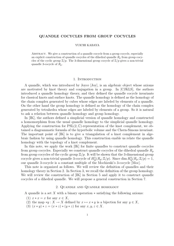
Figure 4. A shadow coloring of (2, p)-torus knot by Rp. (For any x, y, r ∈ Rp.) Then ˜ f satisfies the conditions (1), (2) and (3). So we obtain a quandle k-cocycle. We give an explicit presentation of the 3-cocycle coming from b1b2 ∈ H3(G; Z/p). Let d(x, y) = b2(x, y) − b2(−x, −y) then d is a 2-cocycle. (We can check that d is cohomologous to 2b2.) Then b1b2 is given by [x|y|z] → x · d(y, z). Proposition 6.1. The 3-cocycle coming from b1b2 ∈ H3(G; Z/p) has the following pre- sentation: (x, y, z) → 2z(d(y − x, z − y) + d(y − x, y − z)) (x, y, z ∈ Rp). This is a non-trivial quandle 3-cocycle of Rp.

• Proof. In (5.1), since the map ϕ∗ does not depend on the choice of p ∈ Rp, we let p = 0.

Then we have ϕ(x, y, z) = (0, x, y, z) − (0, x ∗ y, y, z) − (0, x ∗ z, y ∗ z, z) + (0, (x ∗ y) ∗ z, y ∗ z, z) =(0, x, y, z) − (0, 2y − x, y, z) − (0, 2z − x, 2z − y, z) + (0, 2z − 2y + x, 2z − y, z). Rewrite in inhomogeneous notation, this is equal to [x|y − x|z − y] − [2y − x|x − y|z − y] − [2z − x|x − y|y − z] + [2z − 2y + x|y − x|y − z]. Evaluating by b1b2, we have xd(y − x, z − y) − (2y − x)d(x − y, z − y) − (2z − x)d(x − y, y − z) + (2z − 2y + x)d(y − x, y − z) =xd(y − x, z − y) + (2y − x)d(y − x, y − z) + (2z − x)d(y − x, z − y) + (2z − 2y + x)d(y − x, y − z) =2zd(y − x, z − y) + 2zd(y − x, y − z). We can check that this cocycle is non-trivial by evaluating at the cycle given by a coloring

• f the (2, p)-torus knot (Figure 4).
• Since 2 is divisible in Z/p, (x, y, z) → z(d(y − x, z − y) + d(y − x, y − z)) is also a

non-trivial quandle 3-cocycle. It is known that dimFp H3

Q(Rp; Fp) = 1, our cocycle is a

constant multiple of the Mochizuki’s 3-cocycle [Moc].

8

−1 x + y x x + y +1 x

Figure 5. The value of d(x, y). We remark that the cocycle d can be easily understand geometrically. Identify i ∈ Z/p with ζi where ζ = exp(2π√−1/p). Then d(x, y) = −1 if (0, x, x + y) is counterclockwise, d(x, y) = +1 if (0, x, x + y) is clockwise and d(x, y) = 0 otherwise (Figure 5). This interpretation and the equation d(−x, −y) = −d(x, y) make various calculations easy.

• 7. General construction

7.1. Let G be a group. Fix an element h ∈ G. Let Conj(h) = {g−1hg|g ∈ G}. Now Conj(h) has a quandle operation by x ∗ y = y−1xy. Let Z(h) = {g ∈ G|gh = hg} be the centralizer of h in G. Lemma 7.1. As a set Conj(h) ∼ = Z(h)\G by g−1hg ↔ Z(h)g (right coset) From now on we study the quandle structure on Z(h)\G and construct a lift of π : G → Z(h)\G. The quandle structure on Conj(h) induces a quandle operation on Z(h)\G: (g−1

1 hg1) ∗ (g−1 2 hg2) = (g−1 2 hg2)−1(g−1 1 hg1)(g−1 2 hg2)

= (g1g−1

2 hg2)−1h(g1g−1 2 hg2)

↔ Z(h)g1(g−1

2 hg2)

The quandle operation on Z(h)\G lifts to a quandle operation on G by g1 • g2 = h−1g1(g−1

2 hg2)

(g1, g2 ∈ G). We can easily check that • satisfies the quandle axioms and the projection map π : G → Z(h)\G is a quandle homomorphism. Let s : Z(h)\G → G be a section of π (π ◦ s = Id). Since s(x ∗ y) and s(x) • s(y) are in the same coset in Z(h)\G, there exists an element c(x, y) ∈ Z(h) satisfying s(x ∗ y) = c(x, y)s(x) • s(y). Lemma 7.2. If Z(h) is an abelian group, c : X × X → Z(h) is a quandle 2-cocycle. If the cocycle c is cohomologous to zero, we can change the section s to satisfy s(x ∗ y) = s(x) • s(y). Example 7.3. Let G be the dihedral group D2p = h, x|h2 = xp = hxhx = 1 where p is an odd number. Then we have Z(h) = {1, h} and Conj(h) = {x−ihxi|i = 0, 1, . . . , p−1} = {hx2i|i = 0, . . . , p−1}. We can identify x−ihxi ∈ Conj(h) with i ∈ Rp = {0, 1, 2, . . . , p−1}. Define a section s : Z(h)\G → G by Conj(h) ∼ = Z(h)\G

s

− → G ∈ ∈ ∈ x−ihxi ↔ Z(h)xi → hxi

9

Then we have s(Z(h)xi ∗ Z(h)xj) = s(Z(h)x2j−i) = hx2j−i = h−1(hxi)(x−jhxj) = s(Z(h)xi) • s(Z(h)xj). Therefore c(x, y) = 0 for any x, y ∈ Rp. Let G be a group. Fix h ∈ G with hl = 1 (l > 1). We assume that Z(h) is abelian and the 2-cocycle corresponding to G → Z(h)\G is cohomologous to zero. Let s : Z(h)\G → G be a section satisfying s(x ∗ y) = s(x) • s(y). Let f : Gk+1 → A be a normalized group k-cocycle in homogeneous notation. Then f satisfies (1)

k+1

∑

i=0

(−1)if(x0, . . . , xi, . . . , xk+1) = 0, (2) f(gx0, . . . , gxk) = f(x0, . . . , xk) for any g ∈ G (left invariance), (3) f(x0, . . . , xk) = 0 if xi = xi+1 for some i. In the following construction, it is convenient to use a right invariant function. So we replace f(x0, . . . , xk) by f(x−1

0 , . . . , x−1 k ). Define ˜

f : Conj(h)k+1 → A by ˜ f(x0. . . . , xk) =

l−1

∑

i=0

f(his(x0), . . . , his(xk)) for x0, . . . , xk ∈ Conj(h). Proposition 7.4. The function ˜ f satisfies the conditions (1), (2) and (3) of Section 5. Therefore ˜ f gives rise to a quandle k-cocycle of Hk

∆(Conj(h); A) and Hk Q(Conj(h); A).

• Proof. It is clear to satisfy (1) and (3) from the conditions on a normalized group cocycle

in homogeneous notation. We only have to check the second property. ˜ f(x0 ∗ y, . . . , xk ∗ y) =

l−1

∑

i=0

f(his(x0 ∗ y), . . . , his(xk ∗ y)) =

l−1

∑

i=0

f(his(x0) • s(y), . . . , his(xk) • s(y)) =

l−1

∑

i=0

f(hi−1s(x0)(s(y)−1hs(y)), . . . , hi−1s(xk)(s(y)−1hs(y))) =

l−1

∑

i=0

f(hi−1s(x0), . . . , hi−1s(xk)) (right invariance) = ˜ f(x0, . . . , xk)

• 10

Corollary 7.5. If Z(h) is abelian and the 2-cocycle corresponding to G → Z(h)\G is cohomologous to zero, then there is a homomorphism Hn(G; A) → Hn

Q(Conj(h); A)

for any abelian group A. Since there exists a homomorphism from the associated group GConj(h) to G, we have a homomorphism Hn(G; A) → Hn(GConj(h); A) → Hn

Q(Conj(h); A)

from the construction of Section 3.2. I do not know any relation between these homomor- phisms. 7.2. We return to the case of Rp discussed in the previous section. Let G be the dihedral group D2p. Consider the short exact sequence (7.1) 0 → Z/p → D2p → Z/2 → 0. This induces a map H∗(D2p; Z/p) → H∗(Z/p; Z/p)Z/2. We can show that this map is an isomorphism. Consider the Hochschild-Serre spectral sequence of (7.1). Since Ers

2 = Hr(Z/2; Hs(Z/p; Z/p)) = 0 for r > 0, we have Ers ∞ = 0 for

r > 0 and E0s

∞ ∼

= Hs(Z/p; Z/p)Z/2. So we have Hs(D2p; Z/p) ∼ = E0s

∞ ∼

= Hs(Z/p; Z/p)Z/2. Let f be the group 3-cocycle (x, y, z) → x · d(y, z), which was discussed in the previous

• section. This is a Z/2-invariant 3-cocycle of H3(Z/p; Z/p), therefore a 3-cocycle of D2p.

Applying our construction for this group cocycle, we obtain a quandle 3-cocycle of Rp, which is twice the cocycle constructed in the previous section. 7.3. Considering the dual of our construction, we obtain a group cycle represented by a cyclic branched covering along a knot K in the following way. Let X be the quandle Conj(h). Let S be a shadow coloring of a knot diagram D with arc and region color by X. Then a cycle C(S) was defined in Section 4. Now ϕ(C(S)) is a cycle in C∆

3 (X) ⊗Z[GX] Z but not in C∆ 3 (X). Define a map ι : C∆ n (X) → C′ n(G)

by ι(x0, . . . , xn) → (s(x0), . . . , s(xn)). Then ι(ϕ(C(S))) ∈ C′

n(G) is still not a cycle in

general. Let x ∈ X be the color of an arc. Define an arc coloring A ∗ x by (A ∗ x)(a) = A(a) ∗ x, (R ∗ x)(r) = R(r) ∗ x (for any arc a and region r). Then S ∗ x = (A(mi) ∗ x, R ∗ x) is also a shadow coloring. We can show that the sum ι(ϕ(C(S))) + ι(ϕ(C(S ∗ x))) + ι(ϕ(C(S ∗ x2))) + · · · + ι(ϕ(C(S ∗ xl−1))) is a group cycle represented by the l-fold cyclic branched covering along the knot K.

11

7.4. Relative group homology. Let G be a group and H be a subgroup of G. We define the relative group homology Hn(G, H; Z) by the homology of the mapping cone of the map Cn(H) ⊗Z[H] Z → Cn(G) ⊗Z[G] Z. We can compute Hn(G, H; Z) as follows. Lemma 7.6. Let K be the kernel of C0(H\G) → Z. Let · · · → F2 → F1 → K → 0 be a free resolution of K as Z[G]-module. Then Hn(G, H; Z) ∼ = Hn(F∗ ⊗Z[G] Z) for n ≥ 1. The quandle Conj(h) can be identified with Z(h)\G. It is easy to check that the complex C∆

∗ (Z(h)\G) is acyclic and have a Z[G]-module structure. If the following acyclic complex

· · · → C∆

2 (Z(h)\G) → C∆ 1 (Z(h)\G) → Ker(C∆ 0 (Z(h)\G) → Z) → 0

is a projective resolution, H∆

n (Z(h)\G) is isomorphic to the relative group homology

Hn(G, Z(h); Z). References

[Bro] K. Brown, Cohomology of groups, Graduate Texts in Mathematics, 87. Springer-Verlag, New York- Berlin, 1982. [CJKLS] J. S. Carter, D. Jelsovsky, S. Kamada, L. Langford, M. Saito, Quandle cohomology and state- sum invariants of knotted curves and surfaces, Trans. Amer. Math. Soc. 355 (2003), no. 10, 3947– 3989. [Eis1] M. Eisermann, Homological characterization of the unknot, Journal of Pure and Applied Algebra 177 (2003) 131–157. [Eis2] M. Eisermann Knot colouring polynomials, arXiv:GT/0707.3895. [IK] A. Inoue, Y. Kabaya, Quandle homology and complex volume, in preparation. [Joy] D. Joyce, A classifying invariant of knots, the knot quandle, J. Pure Appl. Algebra 23 (1982), no. 1, 37–65. [Kam] S. Kamada, Quandles with good involutions, their homologies and knot invariants, Intelligence of low dimensional topology 2006, 101–108, Ser. Knots Everything, 40, World Sci. Publ., Hackensack, NJ, 2007. [Moc] T. Mochizuki, Some calculations of cohomology groups of fnite Alexander quandles, Journal of Pure and Applied Algebra 179 (2003) 287–330. Osaka City University Advanced Mathematical Institute, 3-3-138 Sugimoto, Sumiyoshi- ku, Osaka, 558-8585, JAPAN E-mail address: kabaya@sci.osaka-cu.ac.jp

12