
SLIDE 1
ST 762 Nonlinear Statistical Models for Univariate and Multivariate Response
Quadratic versus Linear Estimating Equations
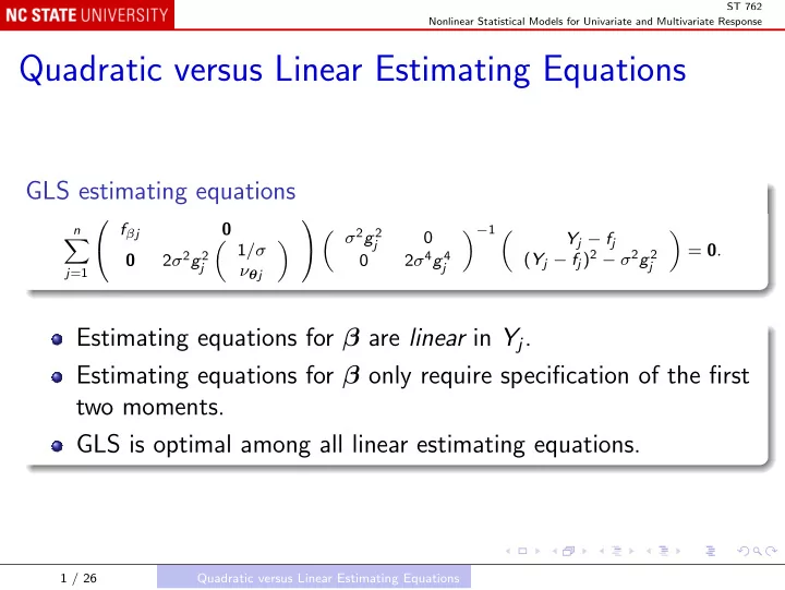
GLS estimating equations
n
- j=1
fβj 2σ2g2
j
1/σ νθj
-
σ2g2
j
2σ4g4
j
−1 Yj − fj (Yj − fj)2 − σ2g2
j
- = 0.
Estimating equations for β are linear in Yj. Estimating equations for β only require specification of the first two moments. GLS is optimal among all linear estimating equations.
1 / 26 Quadratic versus Linear Estimating Equations