Processes What are they? How do we represent them? Scheduling - - PDF document

1

Processes

• What are they? How do we represent

them?

• Scheduling
• Something smaller than a process?

Threads

• Synchronizing and Communicating
• Classic IPC problems

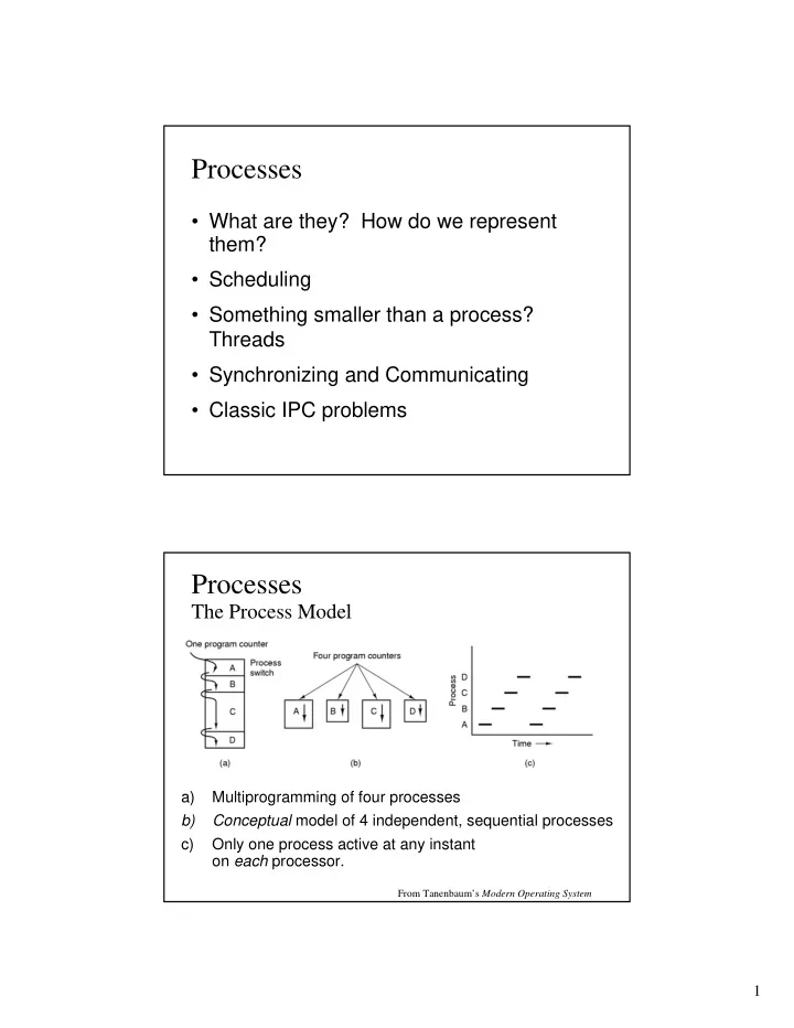
Processes

The Process Model

a) Multiprogramming of four processes b) Conceptual model of 4 independent, sequential processes c) Only one process active at any instant

• n each processor.

From Tanenbaum’s Modern Operating System

2

Process Life Cyle

• Processes are “created”
• They run for a while
• They wait
• They run for a while…
• They die

Process States

From Tanenbaum’s Modern Operating System

3

NT States

Picture from Inside Windows 2000

So what’s a Process?

• What from the OS point of view, is a

process?

• A struct. Sitting on a batch of queues.

4

Implementation of Processes

Fields of a process table entry

From Tanenbaum’s Modern Operating System

Process Creation

Principal events that cause process creation

• A. System start-up
• B. Started from a GUI
• C. Started from a command line
• D. Started by another process

5

Process Termination

Conditions which terminate processes

• 1. Normal exit (voluntary)
• 2. Error exit (voluntary)
• 3. Fatal error (involuntary)
• 4. Killed by another process (involuntary)

From Tanenbaum’s Modern Operating System

Process Hierarchies

• A Process can creates one (or more)

child process.

• Each child can create its own children.
• Forms a hierarchy through ancestry
• Parents have control of their children
• NT processes can give away their

children.

6

Switching from Running

• ne Process to another
• Known as a “Context Switch”
• Requires

– Saving and loading registers – Saving and loading memory maps – Updating Ready List – Flushing and reloading the memory caches – Etc.

Handling Interrupts

Who does what?

7

Need for Multiprogrammng

• How many processes does the computer need

in order to stay “busy”?

Threads

Overview

• Usage
• Model
• Implementation
• Conversions

8

Thread Usage

• Makes it easier to

write programs that have to be ready to do more than one thing at a time using the same data.

Thread Model

• A process consists of

– Open files – Memory management – Code – Global data – Call Stack (includes local data) – Hardware Context:

• Instruction pointer, stack pointer, general registers

9

Thread Model

(continued)

• Each thread has its own

– Stack (includes local variables) – Program counter – General registers (copies)

• A process can have many threads

Thread Implementations

User level thread package

• Implemented as a library in user mode

– Includes code for creating, destroying, switching…

• Often faster for thread creation, destruction and

switching

• Doesn’t require modification of the OS
• If one thread in a process blocks then the whole

process blocks.

• Can only use one processor.

10

Thread Implementations In the Kernel

• An application can have one thread

blocked and still have another thread running.

• The threads can be running on different

processors allowing for true parallelism.

Thread Implementations

User Mode Library In the kernel

From Tanenbaum’s Modern Operating System

11

Hybrid Implementation

Converting Single-threaded to multi- threaded (!!!)

• Not for faint of heart
• Not all libraries are “thread-safe”.
• There may be “global” variables than need

to be “local” to a thread.

12

Scheduling Overview

• Scheduling issues

– What to optimize. Price of a context switch.

• Preemptive vs. non-preemptive
• Three-level scheduling

– Short-term / cpu scheduler – medium-term / memory scheduler – long-term / admission scheduler

• Batch vs. Interactive
• General Algorithms

– FCFS – SJF – SRTN – Round Robin – Priority – Multiple Queue – Guaranteed scheduling – Lottery scheduling – Fair share

• Examples: CTSS, NT, Unix and Linux

CPU Burst

• Processes with long cpu bursts are called compute-bound
• Processes that do a lot of I/O are called I/O-bound

13

Who’s in Charge?

• Who gets to decide when it is time to schedule

the next process to run?

• If the OS allows the currently running process to

get to a good “stopping spot”, the scheduler is non-preemptive.

• If, instead, the OS can switch processes even

while a process is in the middle of its cpu-burst, then the scheduler is preemptive

Scheduling Algorithm Goals

From Tanenbaum’s Modern Operating System

14

First-Come, First-Served (FCFS)

Process Arrival Time Burst Time P1 7 P2 2 4 P3 4 1 P4 5 4

• Non-preemptive
• Average waiting time = (0 + 5 + 7 + 7) / 4 = 4.75
• Average turnaround time = ( 7 + 9 + 8 + 11 ) / 4 = 8.75

P1 P3 P2 P4 7 16 11 12

From Silberchatz’ Operating System Concepts

Shortest Job First (SJF)

Process Arrival Time Burst Time P1 7 P2 2 4 P3 4 1 P4 5 4

• Non-preemptive
• Average waiting time = ( 0 + 6 + 3 + 7 ) / 4 = 4
• Average turnaround time = ( 7 + 10 + 4 + 11 ) / 4 = 8

P1 P3 P2 7 3 16 P4 8 12

Adapted from Silberchatz’ Operating System Concepts

15

Shortest Remaining Time Next (SRTN)

Process Arrival Time Burst Time P1 7 P2 2 4 P3 4 1 P4 5 4

• Preemptive
• Average waiting time = ( 9 + 1 + 0 + 2 ) / 4 = 3
• Average turnaround time = ( 16 + 5 + 1 + 6 ) / 4 = 7

P1 P3 P2 4 2 11 P4 5 7 P2 P1 16

From Silberchatz’ Operating System Concepts

Using “Aging” to Estimate Length of Next CPU Burst

• Useful for both batch or interactive processes.
• Provides an estimate of the next length.
• Can be done by using the length of previous CPU

bursts, using exponential averaging.

: D efine 4. 1 , 3. burst C PU next for the value predicted 2. burst C PU

• f

length actual 1.

1

≤ ≤ = =

+

α α τ n

th n

n t

( )

. 1

1 n n n

t τ α α τ − + =

+

16

Prediction of the Length of the Next CPU Burst

From Silberchatz’ Operating System Concepts

Round Robin

• Each process gets a small unit of CPU time (time

quantum), usually 10-100 milliseconds. After this time has elapsed, the process is preempted and added to the end of the ready queue.

• If there are n processes in the ready queue and the time

quantum is q, then each process gets 1/n of the CPU time in chunks of at most q time units at once. No process waits more than (n-1)q time units.

• Performance

– q large ⇒ FIFO – q small ⇒ q must be large with respect to context switch,

• therwise overhead is too high.

From Silberchatz’ Operating System Concepts

17

Example of RR with Time Quantum = 20

Process Burst Time P1 53 P2 17 P3 68 P4 24

• The Gantt chart is:
• Typically, higher average turnaround than SJF, but better response.

P1 P2 P3 P4 P1 P3 P4 P1 P3 P3 20 37 57 77 97 117 121134 154162

From Silberchatz’ Operating System Concepts

Priority Scheduling

• Each process is explicitly assigned a

priority.

• Each queue may have its own scheduling

strategy.

• No process in a lower priority queue will

run so long as there is a ready process in a higher priority queue.

18

Multi-Queue with Feedback

• Different queues, possibly with different

scheduling algorithms.

• Could use a RR queue for “foreground”

processes and a FCFS queue for “background”.

• Example: CTSS had a multilevel queue

– Each lower priority had a quantum twice as long as the one above. – You moved down in priority if you used up your quantum. – Receiving a carriage-return at the process’s keyboard moved the process to the highest priority.

Guaranteed Scheduling

• What if we want to guarantee that a

process get x% of the CPU? How do we write the scheduler?

• Scheduling algorithm would compute the

ratio of

a) The fraction of CPU time a process has used since the process began b) The fraction of CPU time it is supposed to have.

• The process with the lowest ratio would

run next.

19

Lottery

• Issue lottery tickets.
• The more lottery tickets you have, the

better your chance of “winning”.

• Processes can give (or lend) their tickets

to their children or to other processes.

Fair Share

• If there are 2 users on the machine, how

much of the CPU time should each get?

• In Unix or NT it would depend on who

has more processes (or threads).

• Dividing the time based on the number of

users instead, would be called “a fair share”

20

NT Scheduling

From Tanenbaum’s Modern Operating System

• Priority Inversion:

When a high priority process is prevented from making progress due to a lower priority process.

• High Priority process waits on a resource held by a Low Priority
• process. [By itself this does not constitute a problem.]
• But the low priority process can’t release the resource because

a Medium Priority process is running.

• Here we have one process (medium priority) blocking a higher

priority process.

• How do unix and NT handle this?

Priority Inversion

21

UNIX Scheduler

• Fixed quantum size.
• The running process’s cpu_usage

count is incremented when the clock ticks

• Once per second the cpu_usage is

“aged” and priorities are recomputed

• Priority ≈ base + cpu_usage + nice
• Processes waiting inside the kernel for

i/o to complete have negative (high) priorities, but these drop to “normal” when they return to user space.

From Tanenbaum’s Modern Operating System

Linux 2.4 Scheduler

• Processes are assigned CPU time once each epoch. A

new epoch begins when no ready-to-run job has any cpu time left.

• A process can carry over half its unused CPU time from

the last epoch.

• Priority (known as goodness) is recalculated each time

the scheduler runs.

• Goodness is largely determined by the unused cpu time.
• Preference is given to a process if it uses the same

memory space as the last process (so the memory management cache doesn’t need to be cleared).

• Preference is given in a multiprocessor machine to a

process if it last ran on the current processor. This improves cache hits.

22

Linux 2.6 Scheduler

• 140 levels.

– First 100 are “real time”. Last 40 for “user” – Allows a 5-word bit map to identify occupied levels.

• Active vs. expired arrays. Active array of levels holds processes to

be scheduled

• When user process uses up its quantum it moves to the expired

array.

– Priority is then recalculated based on “interactivity”: – ratio of how much it executed compared to how much it slept. – adjusts priority ±5. – Quantum is based on priority. Better priority has longer quantum.

• (Note: different sources quote different ranges… have to check real source)
• Queues are swapped when no active user process left.

– Like the 2.4 scheduler this allows low priority processes to get a chance.

• Separate structures for each cpu, but migration is possible.

Issues for Multi-level Round Robin Queues

• Quantum

– Fixed size or variable – When / how is it “used up”

• Priority

– How is it determined – When is it modified

23

IPC Overview

• IPC (InterProcess Communication)

– Allows processes to exchange data and synchronize execution

• Issues

– Race Condition – Critical Region / Mutual Exclusion

• Guaranteeing Mutual Exclusion with

– Pure software solutions – Hardware assistance – Common abtractions

• Semaphore
• Monitor
• Other forms of communication.

Race Condition

//Process A //x = x + 1; MOV EAX, x // line 1 INC EAX // line 2 MOV x, EAX // line 3 Scenario 1 Proc A – line 1 Proc B – line 1,2,3 Proc A – line 2,3 Result: 1 // Process B //x = x - 1; MOV EAX, x // line 1 DEC EAX // line 2 MOV x, EAX // line 3 Scenario 2 Proc A – line 1 Proc B – line 1 Proc A – line 2,3 Proc B – line 2,3 Result: -1 x = 0; // Shared memory

24

Critical Region

• Any section of code where shared memory is

accessed or modified

• Conditions for a good solution for avoiding

races:

– No two processes may be in their corresponding critical regions simultaneously (mutual exclusion) – No assumptions to be made about speed or number

• f processes

– No process running outside a critical region may block another process from entering – No process should have to wait forever.

Easy Solution: Disable Interupts

• Eeek!
• Obviously this can only be done in kernel

mode.

• And even in kernel mode it’s not great.
• Especially inefficient and difficult with

multiple processors.

• But sometimes it may be the right (or

simplest) answer.

25

Software Solution: Using a “lock”

int lock = 0; // lock is a shared variable // Call this BEFORE // beginning the // critical region void enterRegion() { // bit spin waiting // for lock while (lock == 1) yield(); lock = 1; } // Call this AFTER // finishing the // critical region void leaveRegion() { lock = 0; }

Software Solution:

Taking Turns

// Call this before // beginning the // critical region void enterRegion(int proc) { // bit spin waiting // for turn while (turn != proc) yield(); } // Call this after // finishing the // critical region void leaveRegion(int proc) { turn = 1 - proc; }

26

Software Solution:

Taking Turns

Process 0

while (TRUE) { enterRegion(0); criticalRegion(); leaveRegion(0); nonCriticalRegion(); }

Process 1

while (TRUE) { enterRegion(1); criticalRegion(); leaveRegion(1); nonCriticalRegion(); }

Software Solution: Peterson’s Solution

int turn; // Will be set before first use bool interested[2]; // Initialized to false void enter_region (int process) { int other = 1 - process; interested[process] = true; turn = process; while (turn == process && interested[other] == true) ; // NOTE: Loop does nothing but check state } void exit_region (int process) { interested[process] = false; }

27

Hardware Solution: Disable Interupts

• Eeek!
• Obviously this can only be done in kernel

mode.

• And even in kernel mode it’s not great.
• Especially inefficient and difficult with

multiple processors.

• But sometimes it may be the right (or

simplest) answer.

Hardware Solution: Atomic Machine Instruction

• Atomic machine instruction

– Instruction that cannot be interrupted

• Test and Set Lock (TSL)

– Test a memory location and set it. – Motorolla 680x0 – Usage: TSL register, memory

– Enter_region: TSL reg, LOCK// Copy LOCK to the register // and set LOCK = 1 CMP reg, 0 // Compare the register with zero. BNE Enter_region // If it wasn’t zero, try again. – Exit_region: MOVE LOCK, 0

• Swap

– Exchanges register with memory. – Intel x86

28

Busy Wait and Priority Inversion

• Busy wait can lead to priority inversion.
• If a high-priority process busy-waits on a

resource held by a low-priority process then the low-priority process will never get to execute.

• Effectively, the low priority process is blocking

the busy-waiting high priority process from ever proceeding.

• Moral: busy-waiting must be used with caution.

Producer / Consumer Problem

• A problem involving two kinds of processes, producers

and consumers, and a shared fixed-sized queue.

• Producers produce things and place them in the queue.
• Consumers take things out of the queue and consume

them.

• What should happen if

– the queue is full when the producer wants to put something in? – The queue is empty when the consumer goes to take something

• ut?
• How do we block the producer / consumer until the right

time and then make sure they get back to work?

29

Sleep and Wakeup

Producer-consumer problem with fatal race condition

From Tanenbaum’s Modern Operating System

Semaphores

• A very widely used primitive for

synchronization.

• Think of it as an abstract data type with just

three operations:

– Constructor / initializer – P(). Attempts to “lock” the semaphore. – V(). Frees the semaphore.

• NEVER access the “value” of a semaphore
• directly. Only access it through the provided
• perations.
• P() and V() are atomic.
• Tannenbaum uses “down()” and “up()”

instead.

• Semaphores come in two flavors:

–

• Binary. Also called Mutex.

–

• Counting. Allows more than one process to

“own the lock” simultaneously.

30

Mutex roughly implemented using TSL

From Tanenbaum’s Modern Operating System

Note that in a real implementation, failing to get the lock on a mutex would put the process on a wait queue. Tanenbaum likes this version because it can be done in user mode.

Counting Semaphores

Can be used to allocating N things. Declare a semaphore S:

int S = N;

Simple conceptual implementation of the operations:

P(S): {

• -S;

if (S < 0) sleep(); } V(S): { ++S; wake(); // Wake one of the waiting processes }

These functions must be “atomic”. And never access the value of the semaphore directly.

31

Semaphores can be tricky…

Process A P(S); P(Q); M V(Q); V(S); Process B P(Q); P(S); M V(S); V(Q)

• Above is one source of error, two processes requesting to

lock a pair of semaphores, but in reverse order.

• Or suppose a programmer fails to use the V operation…
• Or even the P operation!

Using Semaphores

The producer-consumer problem using semaphores

From Tanenbaum’s Modern Operating System

32

Monitor

• High-level synchronization
• primitive. Must be provided by

the language.

• Collection of data and

procedures collected together. (like an OOP class)

• Only one procedure in a

monitor can be active at a time.

• A process that is running in a

monitor procedure can block itself by waiting on a condition variable.

Monitors

From Tanenbaum’s Modern Operating System

33

Condition Variables

• To allow a process to wait within the monitor, a condition

variable must be declared. condition x;

• Condition variables can only be used with the operations wait

and signal.

– The operation

wait(x);

means that the process invoking this operation is suspended until another process invokes

signal(x);

– The signal operation resumes exactly one suspended process. If no process is suspended, then the signal operation has no effect.

• Note that condition variables are also commonly provided with

Mutex libraries.

Schematic View of a Monitor

34

Monitor With Condition Variables Monitors

• Outline of producer-consumer problem with monitors

– only one monitor procedure active at one time – buffer has N slots

From Tanenbaum’s Modern Operating System

35

Monitors

Solution to producer-consumer problem in Java

From Tanenbaum’s Modern Operating System

Monitors

Solution to producer-consumer problem in Java (part 2)

From Tanenbaum’s Modern Operating System

36

Message Passing

• Widely used IPC technique is for the OS to support

sending messages.

– Less “fragile” than semaphores. – Doesn’t require language support (unlike monitors)

• Possible Design Issues:

– Where do we send

• to a process or through a “mailbox”?

– Efficiency

• How many times will the message be sent?
• Maximum size of messages?
• Maximum size of message queue?

– Portability

• Does the interface work with different OS’s?
• Does it work with both single processor and distributed systems?

Using Message Passing

The producer-consumer problem with N messages

From Tanenbaum’s Modern Operating System

37

Barrier

• Here we have several processes that need to synchronize together.
• High level abstractions, such as a barrier, are often convenient to solve

certain types of problems.

Common IPC Mechanisms in Unix and NT

• Semaphores / Mutexes
• Spin Locks
• Signals (unix)
• Pipes. Processes must be related.
• FIFO (aka named pipes). Can be shared by unrelated processes.
• Shared memory.
• Shared Files.
• Message Queues.
• Mail slots (NT) Don’t guarantee delivery. Can send to multiple recipients.
• Remote Procedure Call. The ability to invoke a procedure in another

process.

• Sockets (intended for network communications)
• MPI (Message Passing Interface)

38

Spin Lock

• Suppose when we are trying to get the lock on a resource, we bit spin with

the TSL. What’s the down side?

– We are using up cpu cycles. – On a single core/cpu possibly no one will get to run and free up resource.

• A spin lock is a mechanism where attempting to lock involves

bit-spinning till the lock is gained.

– They may be used when

• you have more than one core/cpu
• and the lock will only be needed for a very short time.
• and the one who has the lock will not get blocked

– Some implementations will switch to a more standard semaphore lock

• If the process/thread that has the lock is currently running
• If bit-spinning turns out to be taking too long
• An optimization to avoid bus traffic is to use a regular read during the bit

spinning and only use the TSL when we believe the lock is free.

Classic IPC Problems

• Producer/Consumer (aka Bounded Buffer)
• Dining Philosophers
• Readers / Writers
• Sleeping Barber

39

Dining Philosophers

• Philosophers eat/think
• Eating needs 2 forks
• Pick one fork at a time
• How to prevent

deadlock

From Tanenbaum’s Modern Operating System

Dining Philosophers

A non-solution

From Tanenbaum’s Modern Operating System

40

Dining Philosophers

From Tanenbaum’s Modern Operating System

Dining Philosophers

From Tanenbaum’s Modern Operating System

41

The Readers and Writers Problem

From Tanenbaum’s Modern Operating System

voi d bef or eReadi ng( ) { P( pr ot ect Count ) ; i f ( ++r c == 1) P( pr ot ect DB) ; V( pr ot ect Count ) ; } voi d af t er Readi ng( ) { P( pr ot ect Count ) ; i f ( - - r c == 0) V( pr ot ect DB) ; V( pr ot ect Count ) ; } t ypedef i nt sem aphor e; sem aphor e pr ot ect Count = 1; / / m ut ex sem aphor e pr ot ect DB = 1; / / m ut ex i nt r c = 0 voi d bef or eW r i t i ng( ) { P( pr ot ect DB) ; } voi d af t er W r i t i ng( ) { V( pr ot ect DB) ; }