[PDF] - PROC NLMIXED SUMMARY Strengths: - Easy to specify non-linear model - PDF Document

SLIDE 1

PROC NLMIXED SUMMARY

Strengths:

Easy to specify non-linear model
Conditional distribution of Y can be almost anything. Normal, Poisson, Binomial,

Gamma, Negative Binomial are built in or you can program your own log- likelihood function

Can estimate non-linear function of parameters with delta method
Easy to generate predicted values with or without EBLUPs

Limitations:

Can’t model autocorrelation
Only two levels (Level 1 and Level 2)
Level 2 random effects must be multivariate normal
Tends to be slow for very large problems

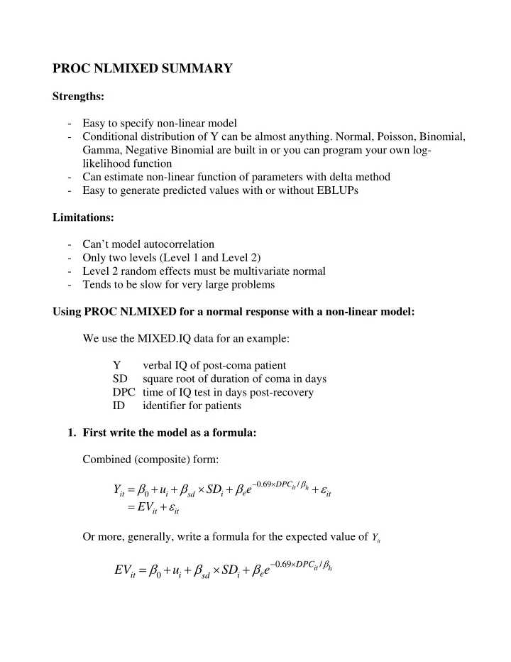
Using PROC NLMIXED for a normal response with a non-linear model: We use the MIXED.IQ data for an example: Y verbal IQ of post-coma patient SD square root of duration of coma in days DPC time of IQ test in days post-recovery ID identifier for patients

1. First write the model as a formula:

Combined (composite) form:

0.69 /

it h

DPC e it i i it sd it it

Y u SD e EV

β

β β β ε ε

− ×

= + + × + + = +

Or more, generally, write a formula for the expected value of

it

Y

0.69 /

it h

DPC e it i i sd

EV u SD e

β

β β β

− ×

= + + × +

SLIDE 2

2

We can use a multilevel approach:

0.69 /

it h

DPC e it i i i i sd

EV B e B SD u

β

β β β

− ×

= + = + × +

2. Specify distributions:

Level 1:

2

| ~ ( , )

it it it

Y EV N EV σ

Level 2:

00

~ (0, )

i

u N τ

3. Classify variables
1. Data:

it i it

Y SD DPC (these are variables in the data set)

Response:

it

Y

Predictors:

i it

SD DPC

2. Basic Parameters:

2 00 e sd h

β β β β σ τ

3. Random variables:

Level 1:

r

it it

Y ε

Level 2:

i

u

4. Computed variables and parameters:

it i

EV B

5. OPTIONAL: Variance Model and Parameters:

e.g. to keep

00

τ positive, we can use a ‘log-parametrization’ in terms

f L, the log of variance.

00

exp( ) L τ =

Note that whatever the value of L may be,

00

τ will be positive.

SLIDE 3

3

Changes to the lists

1. Data: same
2. Basic Parameters: drop

00

τ , add L:

2 e sd h

L β β β β σ

3. Random: same
4. Computed variables and parameters:

00 it i

EV B τ

4. Writing NLMIXED code

Preliminary SORT by ID to play it safe: PROC SORT; DATA = IQ; BY ID; RUN; PROC Statement: PROC NLMIXED DATA = IQ QMAX = 300; PARMS Statement: names and initial values of basic parameters: PARMS b0 = 100 bsd = -2.5 be = - 18 s2 = 8 L = 2 bh = 40; Programming statements: Define all computed variables and parameters: B1 = b0 + u; EV = B1 + bsdSD; + be exp(-0.6931 * DPC / bh); t2 = exp(L);

SLIDE 4

4

MODEL Statement: Randomness at Level 1 Distribution of response conditional on random effects MODEL Y ~ normal(EV, s2); RANDOM Statement: Randomness at Level 2: RANDOM u ~ normal(0, t2) SUBJECT = ID; ESTIMATE Statements: Uses Delta method to estimate functions of parameters: ESTIMATE ’IQ at DC=20 DPC = 365’ b0 + bsd * sqrt(20) + be * exp(-0.69*365/bh); ESTIMATE ’Between Sub SD’ exp(L/2); ESTIMATE ’Within Sub SD’ sqrt(s2); ESTIMATE ’Total SD’ sqrt( t2 + s2 ); ESTIMATE ’Reliability’ t2/( t2 + s2 ); PREDICT Statements: PREDICT EV OUT=OUTDS; run; See output in Appendix

SLIDE 5

5

More than one random effect: Log-Cholesky parametrization of matrix T

Suppose we would like to model both the initial deficit and the long-term level as random and depending on the duration of coma. A Log-Cholesky parametrization

f T ensures that T is a proper variance matrix.

1, First write the model as a formula (we go directly to the multilevel form):

0.69 / 1 1 1 1 1

it h

DPC it i i i i i sd i i i sd

EV B B e B SD u B SD u

β

β β β β

− ×

= + = + × + = + × +

2. Specify distributions:

Level 1:

2

| ~ ( , )

it it it

Y EV N EV σ

(same as before) Level 2:

00 01 1 01 11

~ ,

i i

u N u τ τ τ τ

⎛ ⎞ ⎡ ⎤ ⎡ ⎤ ⎡ ⎤ ⎜ ⎟ ⎢ ⎥ ⎢ ⎥ ⎢ ⎥ ⎜ ⎟ ⎢ ⎥ ⎢ ⎥ ⎜ ⎟ ⎢ ⎥ ⎣ ⎦ ⎣ ⎦ ⎣ ⎦ ⎝ ⎠

Log-Cholesky parametrization of T:

2 2 11 11 10 01 10 00 2 00 00 11 1 00

exp( ) exp( ) c c c c c c L c L τ τ τ = + = = = =

SLIDE 6

6

3. Classify variables
1. Data:

it i it

Y SD DPC (same as before)

Response:

it

Y

Predictors:

i it

SD DPC

2. Basic Parameters:

Expected value:

2 1 1 01 1 sd sd h

L L c β β β β β σ

Variance:

2 1 01

L L c σ

3. Random variables:

Level 1:

r

it it

Y ε

Level 2:

1 i i

u u

4. Computed variables and parameters:

1 00 11 01 00 11 it i i

EV B B c c τ τ τ

4. Writing NLMIXED code

PROC Statement: PROC NLMIXED DATA = IQ QMAX = 300; PARMS Statement: names and initial values of basic parameters: PARMS b0 = 100 b0sd = -2.5 b1 = - 18 b1sd = 0 bh = 40 s2 = 8 L0 = 2

SLIDE 7

7

L1 = 2 c01 = 0 ; Programming statements: Define all computed variables and parameters: B0i = b0 + b0sd * SD + u0; B1i = b1 + b1sd * SD + u1; EV = B0i + B1i * exp(-0.6931 * DPC / bh); c00 = exp(L0); c11 = exp(L1); t00 = c00**2; t01 = c00c01; t11 = c112 + c012; MODEL Statement: Randomness at Level 1 Distribution of response conditional on random effects MODEL Y ~ normal(EV, s2); RANDOM Statement: Randomness at Level 2: RANDOM u0 u1 ~ normal([0, 0], [t00, t01, t11]) SUBJECT = ID; ESTIMATE Statements: Uses Delta method to estimate functions of parameters: ESTIMATE ’IQ at DC=20 DPC = 365’ b0 + b0sd sqrt(20) + b1 * b1sd * sqrt(20) + exp(-0.69*365/bh); PREDICT Statements: PREDICT EV OUT=OUTDS; run;

SLIDE 8

8

Using PROC NLMIXED for multilevel logistic regression:

In dataset: Y binary outcome X1, X2 predictors ID subject identifier SAS code for logistic regression: PROC NLMIXED DATA=dataset; PARMS b0 = 0 b1 = 0 b2 = 0 L = 0; eta = b0 + b1X1 + b2X2 + u; /* linear model / p = 1 / (1 + exp(- eta )); / inverse link function / tau = exp(L); / variance model */ MODEL Y ~ binary( p ); RANDOM u ~ normal ( 0 , tau ) subject = id; run;

SLIDE 9

9

Appendix: SAS code for asymptotic regression

data iq; set mixed.iq; SD = sqrt(DCOMA); DPC = DAYSPC; Y = VIQ; run; proc contents data = iq; run; proc sort data = iq; by id; run; PROC NLMIXED DATA = IQ QMAX = 300; PARMS b0 = 100 bsd = -2.5 be = - 18 s2 = 8 L = 2 bh = 40; B1 = b0 + u; EV = B1 + bsdSD + be exp(-0.6931 * DPC / bh); t2 = exp(L); MODEL Y ~ normal(EV, s2); RANDOM u ~ normal(0, t2) SUBJECT = ID; ESTIMATE 'IQ at DC=20 DPC = 365' b0 + bsd * sqrt(20) + be * exp(-0.69*365/bh); ESTIMATE 'Between Sub SD' exp(L/2); ESTIMATE 'Within Sub SD' sqrt(s2); ESTIMATE 'Total SD' sqrt( t2 + s2 ); ESTIMATE 'Reliability' t2/( t2 + s2 ); PREDICT EV OUT=OUTDS; run;

SLIDE 10

10

/* model with two random effects / PROC NLMIXED DATA = IQ QMAX = 300; PARMS b0 = 100 b0sd = -2.5 b1 = - 18 b1sd = 0 bh = 40 s2 = 8 L0 = 2 L1 = 2 c01 = 0 ; B0i = b0 + b0sd SD + u0; B1i = b1 + b1sd * SD + u1; EV = B0i + B1i * exp(-0.6931 * DPC / bh); c00 = exp(L0); c11 = exp(L1); t00 = c00**2; t01 = c00c01; t11 = c112 + c012; MODEL Y ~ normal(EV, s2); RANDOM u0 u1 ~ normal([0, 0], [t00, t01, t11]) SUBJECT = ID; ESTIMATE 'IQ at DC=20 DPC = 365' b0 + b0sd sqrt(20) + b1 * b1sd * sqrt(20) + exp(-0.69*365/bh); PREDICT EV OUT=OUTDS; run;

SLIDE 11

11

Appendix: Output

T The SA SAS S Sy Syst e st em m 1 17: 31 31 M

M
nd

nday, ay, A Apr i pr i l l 4, 4, 20 2005 05 1 11 Th The N e NLM I XE I XED D Pr Pr oce

cedu

dur e r e S Speci f ci f i c i cat at i on i ons Da Dat a t a Se Set t W W O

RK. I
K. I Q

De Depe pende ndent nt V Var i ar i ab abl e l e Y Y Di Di st st r i b r i but ut i o i on f n f or De Depe pend ndent ent V Var i ar i ab abl e l e N Nor m al m al Ra Rand ndom

m

Ef Ef f e f ect s ct s u u Di Di st st r i b r i but ut i o i on f n f or Ra Rand ndom

m

Ef Ef f e f ect s ct s N Nor m al m al Su Subj bj ect ect V Var i ab i abl e l e I I D O p O pt i t i m i z m i zat at i o i on T n Techni hni qu que e D Dual Q Q uasi - si - Ne Newt wt on

n

I n I nt e t egr a gr at i t i on

n M

e M et h t hod

d

A Adapt i pt i ve ve G a G aus ussi si an an Q Q uadr a dr at u t ur e r e D Di m e i m ens nsi o i ons ns O b O bse ser va r vat i t i on

ns U

s Used 2 295 O b O bse ser va r vat i t i on

ns N

s Not Us Used ed To Tot a t al O l O bser vat vat i o i ons ns 2 295 Su Subj bj ect ect s s 1 170 M a M ax x O bs O bs P Per Su Subj bj ect ect 6 6 Pa Par a r am et m et er er s s 6 6 Q u Q uad adr at r at ur ur e e Poi Poi nt nt s s 1 1 P Par a ar am e m et e t er s r s b0 b0 b bsd be be s2 s2 L L bh bh N NegL egLog

gLi

Li ke ke 1 100

2
2. 5

. 5

18

8 8 2 2 40 40 2 2319

319. 5

. 549 4944 44 I t I t er er at i at i on

n H

Hi st i st or

r y

I t I t er er Ca Cal l s l l s N NegLogLi gLi ke ke Di Di f f f f M a M axG r xG r ad ad Sl o Sl ope pe 1 1 3 3 1

1255. 958

95878 78 1

1063. 5
3. 591

91 1

153. 27

. 2761 61

8971.
71. 38

38 2 2 5 5 11 1180

80. 22

. 2207 07 7

75. 738

73808 08 1

19. 454

45428 28

7
79. 8
9. 878

78 3 3 7 7 1

1155. 506

50688 88 2

24. 713

71383 83 2

24. 841

84186 86

6. 638

63846 46 4 4 9 9 1

1141. 227

22713 13 1

14. 279

27974 74 1

14. 583

58334 34

11. 52

. 5216 16 5 5 11 11 1

1129. 838

83848 48 1

11. 388

38866 66 7

7. 3457

45781 81

2. 317

31747 47 6 6 12 12 1

1114. 946

94653 53 1

14. 891

89195 95 1

13. 763

76307 07

10. 23

. 2398 98 7 7 13 13 1

1101. 451

45149 49 1

13. 495

49504 04 10

10. 00

. 0093 93

11. 03

. 0371 71 8 8 15 15 1

1098. 641

64152 52 2

2. 8099

09974 74 9

9. 1113

11359 59

5. 404

40486 86 9 9 17 17 1

1097. 420

42046 46 1

1. 2210

21063 63

0. 6172

17287 87

1. 442

44217 17 10 10 19 19 1

1097. 090

09021 21 0.

0. 330

33025 25 2

2. 3016

01601 01

0. 285

28551 51 11 11 21 21 1

1097. 041

04147 47

0. 0487

48736 36

0. 5139

13939 39

0. 076

07648 48 12 12 22 22 1

1097. 021

02111 11

0. 0203

20364 64

0. 5890

89048 48

0. 006

00657 57 13 13 24 24 1

1096. 928

92888 88

0. 0922

92221 21 1

1. 2317

31754 54

0. 038

03898 98 14 14 26 26 1

1096. 435

43557 57

0. 4933

93312 12

0. 2750

75048 48

0. 123

12391 91 15 15 28 28 1

1096. 432

43234 34

0. 0032

03233 33

0. 0390

39068 68

0. 005

00573 73 T The he SA SAS S S Syst em 1 17: 3 7: 31 1 M

n

M

nda

day, y, Ap Apr i r i l 4 l 4, 20 2005 05 1 12 Th The N e NLM I XE I XED D Pr Pr oce

cedu

dur e r e I t I t er er at i at i on

n H

Hi st i st or

r y

I t I t er er Ca Cal l s l l s N NegLogLi gLi ke ke Di Di f f f f M a M axG r xG r ad ad Sl o Sl ope pe 16 16 30 30 1

1096. 432

43228 28 0.

0. 000

00006 06

0. 0366

36603 03

0. 000

00007 07 17 17 33 33 1

1096. 426

42693 93

0. 0053

05346 46

0. 3751

75182 82

0. 000

00005 05 18 18 35 35 1

1096. 424

42413 13

0. 0028

02804 04

0. 0175

17598 98

0. 003

00358 58 19 19 37 37 1

1096. 424

42412 12 0.

0. 000

00001 01

0. 0175

17529 29

4. 26E

26E- 6

6

N NO TE O TE: : G CO G CO NV NV c conv

nver

er gen gence ce c cr i t r i t er er i on i on s sat i sf i sf i e i ed. d. F Fi t St St at at i s i st i c t i cs

2
2 L

Log

g Li

Li ke kel i h l i hoo

od

d 2 2192

192. 8

. 8

SLIDE 12

12

AI AI C C ( sm ( sm al al l e l er i r i s bet bet t e t er ) r ) 2 2204

204. 8

. 8 AI AI CC CC ( s ( sm a m al l l l er er i s i s be bet t t t er er ) ) 2 2205

205. 1

. 1 BI BI C C ( sm ( sm al al l e l er i r i s bet bet t e t er ) r ) 2 2223

223. 7

. 7 P Par a ar am e m et er t er E Est i m a i m at e t es St St an andar dar d P Par a ar am e m et er t er Es Est i m t i m at at e e E Er r o r r or r DF DF t V t Val ue ue P Pr > | > | t | Al Al ph pha a Lo Lowe wer r U Uppe pper r G G r ad r adi e i ent nt b b0 102

102. 0

. 02 2 1.

1. 878

8783 3 1 169 5

54. 31

31 < <. 00 . 0001 01

0. 05

9

98. 3
8. 310

104 4 10

105. 7
5. 73

3 -

0. 0
0. 006

0681 81 b bsd sd

1. 1
1. 183

833 3 0.

0. 416

4161 1 1 169

2. 84

84

0. 00

. 0050 50

0. 05
2. 0
2. 004

047 7 -

0. 361

3618 8 -

0. 0
0. 005

0562 62 b be

1
18. 5
8. 587

873 3 2.

2. 923

9235 5 1 169

6. 36

36 < <. 00 . 0001 01

0. 05
2
24. 3
4. 358

585 5 - 1

12.
2. 816

8161 1 0

0. 00

. 0002 0258 58 s s2 2

28. 1
8. 105

050 3.

3. 527

5271 1 1 169 7.

7. 97

97 < <. 00 . 0001 01

0. 05

2

21. 1
1. 142

422 2 3

35. 067

0679 9 0

0. 00

. 0000 0013 13 L L

4. 9
4. 952

526 6 0.

0. 123

1237 7 1 169 4

40. 05

05 < <. 00 . 0001 01

0. 05
4. 7
4. 708

085 5 5.

5. 196

1967 7 -

0. 0
0. 016

1659 59 b bh 4

40. 3
0. 344

446 6 9.

9. 640

6408 8 1 169 4.

4. 18

18 < <. 00 . 0001 01

0. 05

2

21. 3
1. 312

127 7 5

59. 376

3766 6 -

0. 0
0. 017

1753 53 A Addi ddi t i t i ona

nal

l Es Est i m t i m at at es es S St andar d ar d La Label bel E Est i m a i m at e t e Er Er r or r or D DF t t Va Val u l ue e Pr Pr > > | t | t | | A Al pha Low Lower er Up Upper per I Q I Q at at D DC=2 C=20 0 DP DPC = C = 3 365 65 96

96. 69

. 6906 06 1

1. 1682

682 16 169 9 82

82. 7

. 77 7 <. <. 000 0001 1 0.

0. 05

05 94

94. 38

. 3845 45 98

98. 9

. 9966 966 Be Bet we t ween en Su Sub b SD SD 11

11. 89

. 8969 69

0. 7356

356 16 169 9 16

16. 1

. 17 7 <. <. 000 0001 1 0.

0. 05

05 10

10. 44

. 4449 49 13

13. 3

. 3490 490 W i W i t hi t hi n n Sub Sub S SD 5

5. 30

. 3014 14

0. 3327

327 16 169 9 15

15. 9

. 94 4 <. <. 000 0001 1 0.

0. 05

05 4

4. 64

. 6447 47 5

5. 9581

581 To Tot al t al S SD 13

13. 02

. 0247 47

0. 6684

684 16 169 9 19

19. 4

. 49 9 <. <. 000 0001 1 0.

0. 05

05 11

11. 70

. 7051 51 14

14. 3

. 3442 442 Re Rel i a l i abi bi l i t l i t y y

0. 83

. 8343 43 0.

0. 02

02584 584 16 169 9 32

32. 2

. 29 9 <. <. 000 0001 1 0.

0. 05

05

0. 78

. 7833 33

0. 8853

853