
SLIDE 1
Pine Trees, Comas and Migraines: Asymptotic and other functions of - - PowerPoint PPT Presentation
Pine Trees, Comas and Migraines: Asymptotic and other functions of time Non-linear Longitudinal Models with SAS PROC NLMIXED Georges Monette York University georges@yorku.ca www.math.yorku.ca/~georges Summer Programme in Data Analysis June
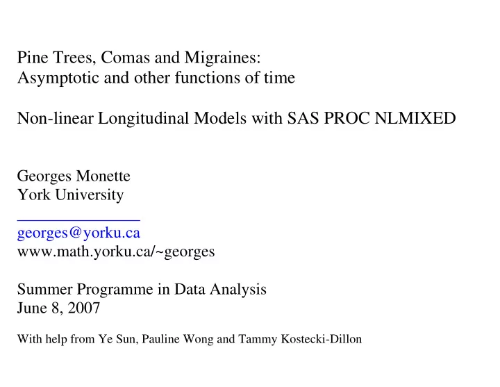
age distance
20 25 30 8 9 10 12 14
M16 M05
8 9 10 12 14
M02 M11
8 9 10 12 14
M07 M08 M03 M12 M13 M14 M09
20 25 30
M15
20 25 30
M06 M04 M01 M10 F10 F09 F06 F01 F05
20 25 30
F07
20 25 30
F02
8 9 10 12 14
F08 F03
8 9 10 12 14
F04 F11
age distance
20 25 30 8 9 10 11 12 13 14
Male
8 9 10 11 12 13 14
Female
DAYSPC PIQ
60 80 100 120 2000 4000 6000 8000 10000 12000
Female
2000 4000 6000 8000 10000 12000
Male
DAYSPC PIQ
60 80 100 120 500 1000 1500 2000 2500
Female
500 1000 1500 2000 2500
Male
PROC NLMIXED DATA = IQ; * PARMS Statement: names and initial values of basic parameters; PARMS b0 = 100 b1 = - 15 a = .1 Ls = 100; /* for log variance of IQ */ * Programming statements; EV = b0 + b1 * exp(-a * time); s2 = exp(Ls); /* ensures variance is positive */ * MODEL Statement (within-subject random model); MODEL IQ ~ normal(EV, s2); * RANDOM Statement: (between-subject random model); * NONE YET; run;
Value Std. Error t value b0 101.190000 2.98566 33.89190 b1 -14.225100 2.15232 -6.60922 a 0.244462 0.12388 1.97337
1 exp{ln(1/ 2)
it sd i i it hrt it
1 exp{ln(1/ 2)
t sd h it it i r i it
2 2
i i t
1 exp{ln(1/ 2)
t sd h it it i r i it
Asymptotic recovery level for ith Subject
1 exp{ln(1/ 2)
sd h it it i r i it
t
1 exp{ln(1/ 2)
t sd h it it i r i it
Asymptotic recovery level for population given DCOMA = 0
Asymptotic recovery level for population given value of DCOMA
1 exp{ln(1/ 2)
sd h it it i r i it
t
1 exp{ln(1/ 2)
t sd h it it i r i it
Initial relative deficit
1 exp{ln(1/ 2) sd h it it i r i it
t
Half recovery time
1 exp{ln(1/ 2)
t sd h it it i r i it
i i t
2 2
Between subject ‘true’ variance
Within-subject variance
1 exp{ln(1/ 2)
t sd h it it i r i it
2 2
i i t
2 2
1 exp{ln(1/ 2)
sd h it it i r i it t
2 2 2 2
it i
2 2
Recap
1 exp{ln(1/ 2)
sd h it it i r i it t
2 2 2 2
it i
2 2
Using PROC NLMIXED
PROC NLMIXED DATA = IQ QMAX = 300 corr ecorr ecov eder; * PARMS Statement: names and initial values of basic parameters; PARMS b0 = 100 bsd = -2.5 b1 = - 18 bhrt = 100 Lg = 2 Ls = 1; * Programming statements: Define all computed variables and parameters; EV = b0 + bsd*SQRTDCOMA + u + b1 * exp(-0.6931 * DAYSPC / bhrt); g2 = exp(Lg); s2 = exp(Ls); * MODEL Statement: Level 1 Distribution of response conditional on random effects; MODEL PIQ ~ normal(EV, s2);
* RANDOM Statement: Randomness at Level 2; RANDOM u ~ normal(0, g2) SUBJECT = ID; * ESTIMATE Statements: Uses Delta method to estimate functions of parameters; ESTIMATE 'IQ at SQRTDCOMA=20 DAYSPC = 365' b0 + bsd * sqrt(20) + b1 * exp(-0.6931 * 365/bh); ESTIMATE 'Between Sub SD' sqrt(g2); ESTIMATE 'Within Sub SD' sqrt(s2); ESTIMATE 'Total SD' sqrt( g2 + s2 ); ESTIMATE 'Reliability' g2/( g2 + s2 ); * PREDICT Statements: generate BLUPs; PREDICT EV OUT=OUTDS; run;
PROC NLMIXED OUTPUT
The N The NLMIXED Procedure MIXED Procedure Specifications Specifications Data Set Data Set WORK.IQ WORK.IQ Dependent Variable Dependent Variable PIQ PIQ Distribution for De Distribution for Dependent Variable pendent Variable Normal Normal Random Effects Random Effects u u Distribution for Random Distribution for Random Effects Effects Normal Normal Subject Variable Subject Variable ID ID Optimization Techniqu Optimization Technique e Dual Dual Quasi-Newton Quasi-Newton Integration Method Integration Method Adaptive Gaussian Adaptive Gaussian Quadrature Quadrature
Dimensions Dimensions Obse Observations Used rvations Used 331 331 Obse Observations Not Used rvations Not Used 0 Tota Total Ob l Observat servations ions 331 331 Subjec Subjects ts 200 200 Max Max Ob Obs s Per Su Per Subject bject 5 5 Parame Paramete ters rs 7 7 Quad Quadra ratu ture Poi re Points ts 1 1 Parameters Parameters b0 b0 bsd bsd b1 b1 bhrt bhrt Lg Lg Ls Ls bh bh NegLogLike NegLogLike 100 -2 100 -2.5 .5
100 100 2 2 1 1 1 3980.10189 1 3980.10189
It Iteration History eration History Iter Calls Iter Calls NegLog NegLogLi Like Diff ke Diff MaxGrad MaxGrad Slope Slope 1 2 1 2 1573.2904 2406.811 1573.2904 2406.811 264.0361 264.0361 -50897.3
2 4 2 4 13 1316.837 16.83773 25 73 256.4527 6.4527 57.36039 57.36039 -157.085
3 6 3 6 1294.2055 22.63224 1294.2055 22.63224 3.743795 3.743795 -23.4729
4 4 8 8 12 1293.89347 93.89347 0. 0.312031 312031 2.446502 2.446502 -0.21904
5 10 5 10 1 1293.65 93.6521 0. 1 0.241366 241366 0.94097 -0.14775 0.94097 -0.14775 6 12 6 12 1293.6239 0.028198 1293.6239 0.028198 0.711704 0.711704 -0.02241
7 13 7 13 1293.58195 0.041954 1293.58195 0.041954 0.859061 -0.01146 0.859061 -0.01146 8 15 8 15 1293.2629 0.319051 1293.2629 0.319051 2.305337 2.305337 -0.06682
9 17 9 17 12 1293.040 93.04005 0. 05 0.222842 222842 0.156794 0.156794 -0.2422
10 10 19 12 19 1293.039 93.03937 0.000 37 0.000684 0.16487 684 0.164873 -0.00071 3 -0.00071 11 22 11 22 12 1292.969 92.96984 0. 84 0.069533 069533 0.996174 0.996174 -0.0007
12 12 24 24 12 1292.951 92.95152 0. 52 0.0183 018315 15 0.056738 0.056738 -0.02862
13 13 26 26 12 1292.951 92.95148 0. 48 0.0000 000047 47 0.043026 0.043026 -0.00007
14 14 30 30 1 1292.93 92.9368 0. 8 0.0146 014676 76 1.084556 1.084556 -0.00003
15 33 15 33 12 1292.528 92.52879 0. 79 0.408005 408005 0.199777 0.199777 -0.0283
16 35 16 35 12 1292.521 92.52165 0 65 0.00714 00714 0.090852 0.090852 -0.0112
17 17 37 37 12 1292.521 92.52132 0. 32 0.0003 000332 32 0.005506 0.005506 -0.00069
18 18 39 39 12 1292.521 92.52132 1. 32 1.671E 671E-6 0.00039
4 -3.45E-6 NOTE: GC NOTE: GCON ONV V conv convergence criterio ergence criterion satisfied. n satisfied.
Fit Statistics Fit Statistics
Log Like keliho lihood
2585.0 2585.0 AIC (s AIC (sma maller i ller is better better) ) 2599.0 2599.0 AICC ( AICC (smaller is bette ller is better) ) 2599.4 2599.4 BIC (s BIC (sma maller i ller is better better) ) 2622.1 2622.1 Para Parameter Es meter Estimates timates Standard Standard Parameter Estima Parameter Estimate Error D te Error DF t Value Pr > |t| t Value Pr > |t| Alpha Lower Alpha Lower Upper Gradient Upper Gradient b0 b0 100.77 100.77 1.9841 1.9841 199 199 50.79 <.0001 50.79 <.0001 0.05 0.05 96.858 96.8584 4 104.68 -0.00002 104.68 -0.00002 bsd - bsd -1.9208 1.9208 0.4147 0.4147 199 -4.6 199 -4.63 <.0001 0.05 3 <.0001 0.05 -2.7386 -1.1
030 -0.00008
b1 - b1 -19.6329 19.6329 1.8 1.8593 93 19 199 -1 9 -10.56 0.56 <.0001 0.05 <.0001 0.05 -23.
2994 -15.9663 -0.0 663 -0.00001 0001 bhrt bhrt 122.60 122.60 2 26.6 .6733 19 733 199 4. 9 4.60 <.0001 60 <.0001 0.05 70.0006 0.05 70.0006 175.20 -1.37E-6 175.20 -1.37E-6 Lg Lg 5.1436 5.1436 0.1 0.1242 19 42 199 9 41.40 <.0001 41.40 <.0001 0.05 4.898 0.05 4.8986 5.3886 0.000394 5.3886 0.000394 Ls Ls 3.8322 3.8322 0.1 0.1261 19 61 199 9 30.39 <.0001 30.39 <.0001 0.05 3.5835 0.05 3.5835 4.0809 0.000307 4.0809 0.000307
Additional Estimates Additional Estimates Standa Standard rd Label Label Es Estimate timate Err Error DF r DF t Value Pr > t Value Pr > |t |t| | Alpha Alpha Lower Lower IQ at SQRTDCOMA IQ at SQRTDCOMA=20 DAYSPC = 365 =20 DAYSPC = 365 92.180 92.1809 1.6019 199 9 1.6019 199 57.54 <.0001 57.54 <.0001 0.05 89.0220 0.05 89.0220 Between Sub SD Between Sub SD 13.0891 0.8131 19 13.0891 0.8131 199 16.10 <.0001 9 16.10 <.0001 0.05 11.4858 0.05 11.4858 Within Sub SD Within Sub SD 6.7945 6.7945 0.42 0.4284 84 199 15.86 199 15.86 <.0001 0. <.0001 0.05 5.9496 05 5.9496 Total SD Total SD 14.7475 14.7475 0.7033 0.7033 199 199 20.97 <.00 20.97 <.0001 0.05 13.3607 01 0.05 13.3607 Reliability Reliability 0.7877 0.7877 0.03281 0.03281 199 24.01 <.0001 199 24.01 <.0001 0.05 0.05 0.72 0.7230 30 Additional Estimates Additional Estimates Label Label Upper Upper IQ at SQRTDCOMA=20 DA IQ at SQRTDCOMA=20 DAYSPC = 365 YSPC = 365 95.3399 95.3399 Betwee Between Su n Sub S b SD D 14.6925 14.6925 Within Within Su Sub SD b SD 7.6393 7.6393 Total SD Total SD 16.1344 16.1344 Reliab Reliability ility 0.8524 0.8524
Fitting the same model to VIQ
VIQ
Standard Standard Parameter Estima Parameter Estimate Error D te Error DF t Value Pr > |t| t Value Pr > |t| Alpha Lower Alpha Lower Upper Gradient Upper Gradient b0 b0 99.9789 99.9789 1.5882 1.5882 199 199 62.95 <.0001 62.95 <.0001 0.05 0.05 96.847 96.8470 0 103.11 -5.93E-6 103.11 -5.93E-6 bsd bsd -0.7085
0.3864 19 64 199 9 -1.83 0.0682
0.05 -1.4705 0.05353 -0.00005 0.05353 -0.00005 b1 - b1 -20.9141 20.9141 3.8 3.8058 19 58 199 - 9 -5.50 <.0001 0.05 .50 <.0001 0.05 -28.
4190 -13.4093 9.09 093 9.098E-6 8E-6 bhrt bhrt 34.2941 34.2941 9.1 9.1768 19 68 199 3. 9 3.74 0.0002 74 0.0002 0.05 16.1978 0.05 16.1978 52.3905 52.3905 -3.6E-6
Lg Lg 5.0568 5.0568 0.1 0.1162 19 62 199 9 43.52 <.0001 43.52 <.0001 0.05 4.827 0.05 4.8277 5.2859 0.000399 5.2859 0.000399 Ls Ls 3.4337 3.4337 0.1 0.1242 19 42 199 9 27.64 <.0001 27.64 <.0001 0.05 3.188 0.05 3.1887 3.6786 -0.00002 3.6786 -0.00002
PIQ
Standard Standard Parameter Estima Parameter Estimate Error D te Error DF t Value Pr > |t| t Value Pr > |t| Alpha Lower Alpha Lower Upper Gradient Upper Gradient b0 b0 100.77 100.77 1.9841 1.9841 199 199 50.79 <.0001 50.79 <.0001 0.05 0.05 96.858 96.8584 4 104.68 -0.00002 104.68 -0.00002 bsd - bsd -1.9208 1.9208 0.4147 0.4147 199 -4.6 199 -4.63 <.0001 0.05 3 <.0001 0.05 -2.7386 -1.1
030 -0.00008
b1 - b1 -19.6329 19.6329 1.8 1.8593 93 19 199 -1 9 -10.56 0.56 <.0001 0.05 <.0001 0.05 -23.
2994 -15.9663 -0.0 663 -0.00001 0001 bhrt bhrt 122.60 122.60 2 26.6 .6733 19 733 199 4. 9 4.60 <.0001 60 <.0001 0.05 70.0006 0.05 70.0006 175.20 -1.37E-6 175.20 -1.37E-6 Lg Lg 5.1436 5.1436 0.1242 199 0.1242 199 41.4 41.40 <.0001 0.05 0 <.0001 0.05 4.8986 4.8986 5.3886 0.000394 5.3886 0.000394 Ls Ls 3.8322 3.8322 0.1 0.1261 19 61 199 9 30.39 <.0001 30.39 <.0001 0.05 3.583 0.05 3.5835 4.0809 0.000307 4.0809 0.000307
PROC NLMIXED SUMMARY
Strengths:
you need a different distribution you can program your own log-likelihood function
Limitations:
Using PROC NLMIXED for a normal response with a non-linear model: We use the MIXED.IQ data for an example: Y verbal IQ of post-coma patient SD square root of duration of coma in days DPC time of IQ test in days post-recovery ID identifier for patients
Combined (composite) form:
1 The expression “G-side” refers to the “G” matrix in PROC MIXED which is specified through the RANDOM statement; R-side random effects are represented in the “R” matrix
specified in the REPEATED statement in PROC MIXED. PROC NLMIXED has no equivalent to the REPEATED statement. The social science literature tends to use T (Greek Tau) to represent G and Σ (Greek Sigma) to represent R.
0.69 /
it h
DPC e it i i it sd it it
Y u SD e EV
β
β β β ε ε
− ×
= + + × + + = +
Note: In contrast with linear model formula (e.g. in PROC GLM or PROC MIXED), this formula contains BOTH parameters and
exactly one parameter that multiplies the carrier. With PROC NLMIXED, we don’t have to write the formula in one line. We can use a sequence of “DATA” step statements. We can write a formula for the expected value of Y:
0.69 /
it h
DPC e it i i sd
EV u SD e
β
β β β
− ×
= + + × +
Or we can use a multilevel approach:
0.69 /
[within subject model] [between subject model]
it h
DPC e it i i i i sd
EV B e B SD u
β
β β β
− ×
= + = + × +
Level 1:
2
| ~ ( , )
it it it
Y EV N EV σ
Level 2:
00
~ (0, )
i
u N τ
2
(these are variables in the data set)
it i it
Y SD DPC
Response:
it
Y
Predictors:
i it
SD DPC
2 00 e sd h
β β β β σ τ
Level 1:
it it
Y ε
Level 2:
i
u
it i
EV B
e.g. to keep
00
τ positive, we can use a ‘log-parametrization’ in terms of L, the log of variance.
00
exp( ) L τ =
Whatever the value of L may be,
00
τ will be positive.
Changes to the lists
00
τ , add L:
2
3
e sd h
L β β β β σ
00 it i
EV B τ
Preliminary SORT by ID to play it safe: PROC SORT; DATA = IQ; BY ID; RUN; PROC Statement: PROC NLMIXED DATA = IQ QMAX = 300; PARMS Statement: names and initial values of basic parameters: PARMS b0 = 100 bsd = -2.5 be = - 18 s2 = 8 L = 2 bh = 40; Programming statements: Define all computed variables and parameters: B1 = b0 + u; EV = B1 + bsd*SD; + be * exp(-0.6931 * DPC / bh);
4
5
t2 = exp(L); MODEL Statement: Randomness at Level 1 Distribution of response conditional on random effects MODEL Y ~ normal(EV, s2); RANDOM Statement: Randomness at Level 2: RANDOM u ~ normal(0, t2) SUBJECT = ID; ESTIMATE Statements: Uses Delta method to estimate functions of parameters: ESTIMATE ’IQ at DC=20 DPC = 365’ b0 + bsd * sqrt(20) + be * exp(-0.69*365/bh); ESTIMATE ’Between Sub SD’ exp(L/2); ESTIMATE ’Within Sub SD’ sqrt(s2); ESTIMATE ’Total SD’ sqrt( t2 + s2 ); ESTIMATE ’Reliability’ t2/( t2 + s2 ); PREDICT Statements: PREDICT EV OUT=OUTDS; run; See output in Appendix
More than one random effect: Log-Cholesky parametrization of “G” matrix
Suppose we would like to model both the initial deficit and the long-term level as random and depending on the duration of
1, First write the model as a formula (we go directly to the multilevel form):
0.69 / 1 1 1 1 1
it h
DPC it i i i i i sd i i i sd
EV B B e B SD u B SD u
β
β β β β
− ×
= + = + × + = + × +
Level 1:
2
| ~ ( , )
it it it
Y EV N EV σ
(same as before) Level 2:
00 01 1 01 11
~ ,
i i
u N u τ τ τ τ
⎛ ⎞ ⎡ ⎤ ⎡ ⎤ ⎡ ⎤ ⎜ ⎟ ⎢ ⎥ ⎢ ⎥ ⎢ ⎥ ⎜ ⎟ ⎢ ⎥ ⎢ ⎥ ⎜ ⎟ ⎢ ⎥ ⎣ ⎦ ⎣ ⎦ ⎣ ⎦ ⎝ ⎠ 6
Log-Cholesky parametrization of T:
2 11 11 01 10 11 2 2 00 00 10 11 1 00
exp( ) exp( ) c c c c c c L c L τ τ τ = = = + = =
(same as before)
it i it
Y SD DPC
Response:
it
Y
Predictors:
i it
SD DPC
Expected value:
2 1 1 01 1 sd sd h
L L c β β β β β σ
Variance:
2 1
L
1
L c σ
Level 1:
it it
Y ε
Level 2:
1 i i
u u
7
1 00 11 01 00 11 it i i
EV B B c c τ τ τ
PROC Statement: PROC NLMIXED DATA = IQ QMAX = 300; PARMS Statement: names and initial values of basic parameters: PARMS b0 = 100 b0sd = -2.5 b1 = - 18 b1sd = 0 bh = 40 s2 = 8 L0 = 2 L1 = 2 c01 = 0 ; Programming statements: Define all computed variables and parameters: B0i = b0 + b0sd * SD + u0; B1i = b1 + b1sd * SD + u1; EV = B0i + B1i * exp(-0.6931 * DPC / bh);
8
9
c00 = exp(L0); c11 = exp(L1); t00 = c00**2 + c01**2; t01 = c11*c01; t11 = c11**2; MODEL Statement: Randomness at Level 1 Distribution of response conditional on random effects MODEL Y ~ normal(EV, s2); RANDOM Statement: Randomness at Level 2: RANDOM u0 u1 ~ normal([0, 0], [t00, t01, t11]) SUBJECT = ID; ESTIMATE Statements: Uses Delta method to estimate functions of parameters: ESTIMATE ’IQ at DC=20 DPC = 365’ b0 + b0sd * sqrt(20) + b1 * b1sd * sqrt(20) + exp(-0.69*365/bh); PREDICT Statements: PREDICT EV OUT=OUTDS; run;
10
Using PROC NLMIXED for multilevel logistic regression:
In dataset: Y binary outcome X1, X2 predictors ID subject identifier SAS code for logistic regression: PROC NLMIXED DATA=dataset; PARMS b0 = 0 b1 = 0 b2 = 0 L = 0; eta = b0 + b1*X1 + b2*X2 + u; /* linear model */ p = 1 / (1 + exp(- eta )); /* inverse link function */ tau = exp(L); /* variance model */ MODEL Y ~ binary( p ); RANDOM u ~ normal ( 0 , tau ) subject = id; run;
11
Appendix: SAS code for asymptotic regression
data iq; set mixed.iq; SD = sqrt(DCOMA); DPC = DAYSPC; Y = VIQ; run; proc contents data = iq; run; proc sort data = iq; by id; run; PROC NLMIXED DATA = IQ QMAX = 300; PARMS b0 = 100 bsd = -2.5 be = - 18 s2 = 8 L = 2 bh = 40; B1 = b0 + u; EV = B1 + bsd*SD + be * exp(-0.6931 * DPC / bh); t2 = exp(L); MODEL Y ~ normal(EV, s2); RANDOM u ~ normal(0, t2) SUBJECT = ID; ESTIMATE 'IQ at DC=20 DPC = 365' b0 + bsd * sqrt(20) + be * exp(-0.69*365/bh);
t11 = c11**2;
12
ESTIMATE 'Between Sub SD' exp(L/2); ESTIMATE 'Within Sub SD' sqrt(s2); ESTIMATE 'Total SD' sqrt( t2 + s2 ); ESTIMATE 'Reliability' t2/( t2 + s2 ); PREDICT EV OUT=OUTDS; run; /* model with two random effects */ PROC NLMIXED DATA = IQ QMAX = 300; PARMS b0 = 100 b0sd = -2.5 b1 = - 18 b1sd = 0 bh = 40 s2 = 8 L0 = 2 L1 = 2 c01 = 0 ; B0i = b0 + b0sd * SD + u0; B1i = b1 + b1sd * SD + u1; EV = B0i + B1i * exp(-0.6931 * DPC / bh); c00 = exp(L0); c11 = exp(L1); t00 = c00**2 + c01**2; t01 = c11*c01;
13
MODEL Y ~ normal(EV, s2); RANDOM u0 u1 ~ normal([0, 0], [t00, t01, t11]) SUBJECT = ID; ESTIMATE 'IQ at DC=20 DPC = 365' b0 + b0sd * sqrt(20) + b1 * b1sd * sqrt(20) + exp(-0.69*365/bh); PREDICT EV OUT=OUTDS; run;
14
Appendix: Output
The The NL NLMIX MIXED ED Pro Proced cedure ure Sp Speci ecific ficati ations
Dat Data S a Set et W WORK ORK.IQ .IQ Dep Depend endent ent Va Varia riable ble Y Y Dis Distri tribut bution ion fo for D r Depe epende ndent nt Var Variab iable le N Norm
al Ran Random dom Ef Effec fects ts u u Dis Distri tribut bution ion fo for R r Rand andom
Effect ects s N Norm
al Sub Subjec ject V t Vari ariabl able e I ID Opt Optimi imizat zation ion Te Techn chniqu ique e D Dual ual Qu Quasi asi-Ne
wton Int Integr egrati ation
Method hod A Adap daptiv tive G e Gaus aussia sian Q Quad uadrat rature ure Dim Dimens ension ions Obs Observ ervati ations
Used ed 29 295 Obs Observ ervati ations
Not U t Used sed Tot Total al Obs Observ ervati ations
29 295 Sub Subjec jects ts 17 170 Max Max Ob Obs P s Per er Sub Subjec ject t 6 Par Parame ameter ters s 6 Qua Quadra dratur ture P e Poin
ts 1 Par Parame ameter ters b0 b0 b bsd sd be be s2 s2 L L bh bh Neg NegLog LogLik Like 1 100 00
.5
18 8 8 2 2 40 40 231 2319.5 9.5494 4944 Ite Iterat ration ion Hi Histo story ry Ite Iter r Cal Calls ls Neg NegLog LogLik Like e Dif Diff f Max MaxGra Grad d S Slop lope 1 1 3 3 125 1255.9 5.9587 5878 8 1 1063 063.59 .591 1 1 153. 53.276 2761 1 -
8971.3 1.38 2 2 5 5 11 1180. 80.220 2207 7 7 75.7 5.7380 3808 8 1 19.4 9.4542 5428 8
.878 3 3 7 7 115 1155.5 5.5068 0688 8 2 24.7 4.7138 1383 3 2 24.8 4.8418 4186 6 -
6.6384 3846 4 4 9 9 114 1141.2 1.2271 2713 3 1 14.2 4.2797 7974 4 1 14.5 4.5833 8334 4 -
11.521 5216 5 5 11 11 112 1129.8 9.8384 3848 8 1 11.3 1.3886 8866 6 7 7.34 .34578 5781 1 -
2.3174 1747 6 6 12 12 111 1114.9 4.9465 4653 3 1 14.8 4.8919 9195 5 1 13.7 3.7630 6307 7 -
10.239 2398 7 7 13 13 110 1101.4 1.4514 5149 9 1 13.4 3.4950 9504 4 10. 10.009 0093 3 -
11.037 0371
15
8 8 15 15 109 1098.6 8.6415 4152 2 2 2.80 .80997 9974 4 9 9.11 .11135 1359 9 -
5.4048 0486 9 9 17 17 109 1097.4 7.4204 2046 6 1 1.22 .22106 1063 3 0 0.61 .61728 7287 7 -
1.4421 4217 1 10 19 19 109 1097.0 7.0902 9021 1 0.3 0.3302 3025 5 2 2.30 .30160 1601 1 -
0.2855 8551 1 11 1 21 21 109 1097.0 7.0414 4147 7 0 0.04 .04873 8736 6 0 0.51 .51393 3939 9 -
0.0764 7648 1 12 2 22 22 109 1097.0 7.0211 2111 1 0 0.02 .02036 0364 4 0 0.58 .58904 9048 8 -
0.0065 0657 1 13 3 24 24 109 1096.9 6.9288 2888 8 0 0.09 .09222 2221 1 1 1.23 .23175 1754 4 -
0.0389 3898 1 14 4 26 26 109 1096.4 6.4355 3557 7 0 0.49 .49331 3312 2 0 0.27 .27504 5048 8 -
0.1239 2391 1 15 5 28 28 109 1096.4 6.4323 3234 4 0 0.00 .00323 3233 3 0 0.03 .03906 9068 8 -
0.0057 0573 1 16 6 30 30 109 1096.4 6.4322 3228 8 0.0 0.0000 0006 6 0 0.03 .03660 6603 3 -
0.0000 0007 1 17 7 33 33 109 1096.4 6.4269 2693 3 0 0.00 .00534 5346 6 0 0.37 .37518 5182 2 -
0.0000 0005 1 18 8 35 35 109 1096.4 6.4241 2413 3 0 0.00 .00280 2804 4 0 0.01 .01759 7598 8 -
0.0035 0358 1 19 9 37 37 109 1096.4 6.4241 2412 2 0.0 0.0000 0001 1 0 0.01 .01752 7529 9 -
4.26E- 6E-6 NO NOTE: TE: GC GCONV ONV co conve nverge rgence nce cr crite iterio rion s n sati atisfi sfied. ed. Fi Fit S t Stat tatist istics ics
Log Li Likel keliho ihood
21 2192. 92.8 AIC AIC (s (smal maller ler is is be bette tter) r) 22 2204. 04.8 AIC AICC ( C (sma smalle ller i r is b s bett etter) er) 22 2205. 05.1 BIC BIC (s (smal maller ler is is be bette tter) r) 22 2223. 23.7 Pa Param ramete eter E r Esti stimat mates es St Stand andard ard Pa Param ramete eter r Est Estima imate te Er Error ror DF DF t t Va Value lue P Pr > r > |t |t| | Al Alpha pha L Lowe
r Upp Upper er Gr Gradi adient ent b0 b0 1 102. 02.02 02 1.8 1.8783 783 169 169 54 54.31 .31 <. <.000 0001 1 0 0.05 .05 98. 98.310 3104 4 1 105. 05.73 73 -0
.00681 681 bs bsd d
.1833 33 0.4 0.4161 161 169 169
.84 0. 0.005 0050 0 0 0.05 .05
0047 7 -0
.3618 18 -0
.00562 562 be be
.5873 73 2.9 2.9235 235 169 169
.36 <. <.000 0001 1 0 0.05 .05 -
24.358 3585 5 -12
.8161 61 0. 0.000 000258 258 s2 s2 28 28.10 .1050 50 3.5 3.5271 271 169 169 7 7.97 .97 <. <.000 0001 1 0 0.05 .05 21. 21.142 1422 2 35 35.06 .0679 79 0. 0.000 000013 013 L L 4 4.95 .9526 26 0.1 0.1237 237 169 169 40 40.05 .05 <. <.000 0001 1 0 0.05 .05 4. 4.708 7085 5 5 5.19 .1967 67 -0
.01659 659 bh bh 40 40.34 .3446 46 9.6 9.6408 408 169 169 4 4.18 .18 <. <.000 0001 1 0 0.05 .05 21. 21.312 3127 7 59 59.37 .3766 66 -0
.01753 753 Ad Addit dition ional al Est Estima imates tes Sta Standa ndard rd Lab Label el E Esti stimat mate e Err Error
DF DF t t Val Value ue Pr Pr > > |t| |t| Alp Alpha ha Lo Lower wer U Uppe pper IQ IQ at at DC= DC=20 20 DPC DPC = = 365 365 96. 96.690 6906 6 1 1.16 .1682 82 1 169 69 82. 82.77 77 <.0 <.0001 001 0. 0.05 05 9 94.3 4.3845 845 98. 98.996 9966 Bet Betwee ween S n Sub ub SD SD 11. 11.896 8969 9 0 0.73 .7356 56 1 169 69 16. 16.17 17 <.0 <.0001 001 0. 0.05 05 1 10.4 0.4449 449 13. 13.349 3490 Wit Within hin Su Sub S b SD D 5. 5.301 3014 4 0 0.33 .3327 27 1 169 69 15. 15.94 94 <.0 <.0001 001 0. 0.05 05 4.6 4.6447 447 5. 5.958 9581
16
Tot Total al SD SD 13. 13.024 0247 7 0 0.66 .6684 84 1 169 69 19. 19.49 49 <.0 <.0001 001 0. 0.05 05 1 11.7 1.7051 051 14. 14.344 3442 Rel Reliab iabili ility ty 0. 0.834 8343 3 0. 0.025 02584 84 1 169 69 32. 32.29 29 <.0 <.0001 001 0. 0.05 05 0.7 0.7833 833 0. 0.885 8853