problems for ivan corwin s oops lectures read this first
play

Problems for Ivan Corwins OOPS lectures Read this first: Problems - PDF document

Problems for Ivan Corwins OOPS lectures Read this first: Problems should be completed by groups of students and submitted by 14:00UTC the next day to the TAs. Please identify the members of your group. The TAs will collate and select the


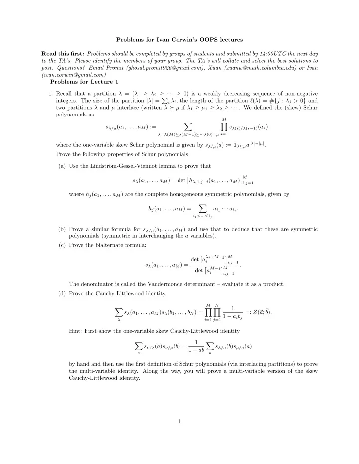
  1. Problems for Ivan Corwin’s OOPS lectures Read this first: Problems should be completed by groups of students and submitted by 14:00UTC the next day to the TA’s. Please identify the members of your group. The TA’s will collate and select the best solutions to post. Questions? Email Promit (ghosal.promit926@gmail.com), Xuan (xuanw@math.columbia.edu) or Ivan (ivan.corwin@gmail.com) Problems for Lecture 1 1. Recall that a partition λ = ( λ 1 ≥ λ 2 ≥ · · · ≥ 0) is a weakly decreasing sequence of non-negative integers. The size of the partition | λ | = � i λ i , the length of the partition ℓ ( λ ) = # { j : λ j > 0 } and two partitions λ and µ interlace (written λ � µ if λ 1 ≥ µ 1 ≥ λ 2 ≥ · · · . We defined the (skew) Schur polynomials as M � � s λ/µ ( a 1 , . . . , a M ) := s λ ( s ) /λ ( s − 1) ( a s ) s =1 λ = λ ( M ) � λ ( M − 1) �··· λ (0)= µ where the one-variable skew Schur polynomial is given by s λ/µ ( a ) := 1 λ � µ a | λ |−| µ | . Prove the following properties of Schur polynomials (a) Use the Lindstr¨ om-Gessel-Viennot lemma to prove that � M � s λ ( a 1 , . . . , a M ) = det h λ i + j − i ( a 1 , . . . , a M ) i,j =1 where h j ( a 1 , . . . , a M ) are the complete homogeneous symmetric polynomials, given by � a i 1 · · · a i j . h j ( a 1 , . . . , a M ) = i 1 ≤···≤ i j (b) Prove a similar formula for s λ/µ ( a 1 , . . . , a M ) and use that to deduce that these are symmetric polynomials (symmetric in interchanging the a variables). (c) Prove the bialternate formula: � M a λ j + M − j � det i i,j =1 s λ ( a 1 , . . . , a M ) = . � M a M − j � det i i,j =1 The denominator is called the Vandermonde determinant – evaluate it as a product. (d) Prove the Cauchy-Littlewood identity M N 1 � � � a ; � s λ ( a 1 , . . . , a M ) s λ ( b 1 , . . . , b N ) = =: Z ( � b ) . 1 − a i b j λ i =1 j =1 Hint: First show the one-variable skew Cauchy-Littlewood identity 1 � � s ν/λ ( a ) s ν/µ ( b ) = s λ/κ ( b ) s µ/κ ( a ) 1 − ab ν κ by hand and then use the first definition of Schur polynomials (via interlacing partitions) to prove the multi-variable identity. Along the way, you will prove a multi-variable version of the skew Cauchy-Littlewood identity. 1
  2. (e) The Schur process on � � � λ = ∅ = λ (0) � λ (1) � · · · λ ( M ) � · · · λ ( M + N − 1) � λ ( M + N ) = ∅ is given by M N b ( � a ; � b ) − 1 � � P � λ ) = Z ( � s λ ( s ) /λ ( s − 1) ( a s ) s λ ( M + N − s ) /λ ( M + N − s +1) ( b s ) . a ; � s =1 s =1 a ; � Consider geo( � b ) random walks Y i , i ≥ 1 from Y i (0) = − i to Y i ( M + N ) = − i . Condition them on non-touching and let λ i ( s ) = Y i ( s ) + i . Show that the induced measure on � λ is precisely the above Schur process. (f) Prove that the marginal distribution of λ ( M ) under the above Schur process is given by the Schur measure a,� b ) − 1 s λ ( � a ) s λ ( � b ( λ ) = Z ( � b ) . P � a ; � What can you say about the law of other marginals (i.e., λ ( s ) for any other s )? 2. Consider a measure P supported on N -element subsets Y = { y 1 , . . . , y N } of a finite set Ω (with | Ω | ≥ N ). Define the k th correlation function � � ρ k ( x 1 , . . . , x k ) := P Y such that { x 1 , . . . , x k } ⊂ Y where we assume all x i are distinct. A P is called determinantal if there exists a kernel K : Ω × Ω → R (or a real valued matrix with rows and columns indexed by Ω) such that for all k , � k � ρ k ( x 1 , . . . , x k ) = det K ( x i , x j ) i,j =1 . Prove that for any S ⊂ Ω, P ( Y ∩ S = ∅ ) = det(1 − K ) S where ∅ is the empty set, 1 is the identity matrix, and det( M ) S means to evaluate the determinant of the | S | × | S | matrix made up entries M i,j for i and j in S . Along the way in proving this you will need to prove the following expansion formula ∞ ( − 1) k � k � � � det( I − K ) S = 1 + det K ( x i , x j ) i,j =1 . k ! k =1 x 1 ,...,x k ∈ S Notice that even though the sum over k is to infinity, it really terminates because eventually all matrices have determinant 0. 3. Consider a measure P N on size N subsets of Z of the form � N � N � i,j =1 · det � P N ( x 1 , . . . , x N ) = c N det φ i ( x j ) ψ i ( x j ) i,j =1 where φ 1 , . . . , φ N , ψ 1 , . . . , ψ N : Z → C are functions such that the Gram matrix � G i,j := φ i ( x ) ψ j ( x ) x ∈ Z has finite entries for 1 ≤ i, j ≤ N , and c N is a constant needed to normalize the measure to sum to 1. Prove that P N is determinantal with kernel N � φ i ( x )[ G − t ] i,j ψ j ( y ) K ( x, y ) = i,j =1 where G − t means the transpose of the inverse of the Gram matrix. Here is a sketch for a proof of this fact – please fill in the details. 2

  3. � N � • Prove that the normalizing constant c N = N ! det G i,j i,j =1 and hence conclude that G is invert- ible. • Prove that there exist matrices A and B such that AGB t = I . Thus, if we define Φ k ( x ) = � N ℓ =1 A kℓ φ ℓ ( x ) and Ψ k ( y ) = � N ℓ =1 B kℓ ψ ℓ ( y ) for 1 ≤ k ≤ N , the Φ and Ψ are biorthogonal in the sense that � x Φ i ( x )Ψ j ( x ) = 1 i = j . • Show that the n -th correlation function can be expressed in terms of the Φ k and Ψ k as 1 � N � N � � � ρ n ( x 1 , . . . , x n ) = det Φ i ( x j ) i,j =1 det Ψ i ( x j ) i,j =1 . ( N − n )! x n +1 ,...,x N • Use the Cauchy-Binet formula to conclude the desired result. 4. Apply the previous formula to the bialternant formula for Schur polynomials to show that the Schur measure is determinantal. Prove Okounkov’s formula: Choose λ from the Schur measure M N 1 a,� b ) − 1 s λ ( � a ) s λ ( � a ; � � � b ( λ ) = Z ( � b ) , where Z ( � b ) = . P � a ; � 1 − a i b j i =1 j =1 Then ˜ � � Y = λ i − i + 1 / 2 i ≥ 1 is a determinantal point process on Z + 1 / 2 with kernel K ( i, j ) defined by the generating series a ; v ) Z ( � b ; w − 1 ) K ( i, j ) v i w − j = Z ( � � k . � � � w/v Z ( � b ; v − 1 ) Z ( � a ; w ) i,j ∈ Z +1 / 2 k =1 / 2 , 3 / 2 , ··· Along the way, you should prove a double-contour integral formula for K ( i, j ) from which the generating function identity follows from Cauchy’s residue theorem. In the special case where M = N and all a i = b j = q , the double-contour integral formula should simplify to √ vw 1 � � � (1 − q/v )(1 − qw ) � N v − i − 1 w j − 1 dvdw (2 π √− 1) 2 K ( i, j ) = v − w (1 − qv )(1 − q/w ) where both the v and w contours are circles that contain q and do not contain 1, and the v contour also entirely contains the w contour. Problems for Lecture 2 1. Consider a line ensemble with k fixed starting points and k fixed ending point, and a bounding curve above and below (as in the figure with k = 2 and the black dots representing the starting and ending points). The ensemble is defined as the uniform distribution on all non-touching paths which are integer valued, piece-wise constant, non-decreasing and connect the starting and ending points, without touching the bounding curves. On the right of the figure we illustrate a jump for the Metropolis Markov chain which chooses a line, a location and then randomly moves the value up or down by 1, provided the update does not violate the conditions set out. Show that this update converges to the uniform distribution. Use this to prove the monotone coupling with respect to different starting and ending points, and bounding curves. 2. Give an example of a discrete random walk which when conditioned to form a bridge violates monotone coupling. Specifically, provide an example of a time homogeneous random walk whose measure, when conditioned to go from 0 to 0, versus from 0 to 1 is not stochastically ordered. 3. Consider a Brownian bridge B : [0 , 1] → R with B (0) = B (1) = 0. Let M [0 , 1 / 2] = max x ∈ [0 , 1 / 2] B ( x ). Use a “no big max” type argument to prove that P ( M [0 , 1 / 2] ≥ s ) ≤ 2 P ( B (1 / 2) ≥ s/ 2). 3

  4. 4. Prove that a Brownian bridge B : [0 , 1] → R with B (0) = B (1) = 0 almost surely has a unique maximizer. Hint: Let I and J be intervals with rational endpoint I = [ i 1 , i 2 ], J = [ j 1 , j 2 ] with i 1 < i 2 < j 1 < j 2 and let E I,J be the event that the maximum of B on I and of B on J are equal. Then the event of non-uniqueness of the maximizer is equal to the countable union of events E I,J where I and J range over the countable number of ordered rational intervals I and J in [0 , 1]. Since this is a countable union, if we can show that the probability of each E I,J is zero, we will be done. Prove that using the Gibbs property for the Brownian bridge. 5. Fill in the details in the proof of the following result: The probability that the maximizer of the Airy 2 process minus a parabola is outside [ − R, R ] is of order e − cR 3 . Use the Gibbs property and a union bound. You may also use the upper and lower tail bounds for the Tracy-Widom GUE distribution (the one-point distribution for the Airy 2 process). 4

Download Presentation
Download Policy: The content available on the website is offered to you 'AS IS' for your personal information and use only. It cannot be commercialized, licensed, or distributed on other websites without prior consent from the author. To download a presentation, simply click this link. If you encounter any difficulties during the download process, it's possible that the publisher has removed the file from their server.

Recommend


More recommend