Homework 1: Gibbsian Line Ensembles Lecturer: Ivan Corwin TA: Xuan - PDF document

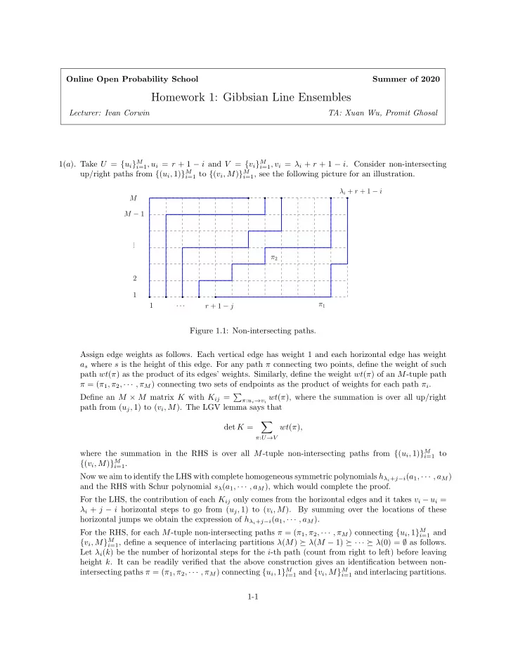
Online Open Probability School Summer of 2020 Homework 1: Gibbsian Line Ensembles Lecturer: Ivan Corwin TA: Xuan Wu, Promit Ghosal 1( a ) . Take U = { u i } M i =1 , u i = r + 1 − i and V = { v i } M i =1 , v i = λ i + r + 1 − i . Consider non-intersecting up/right paths from { ( u i , 1) } M i =1 to { ( v i , M ) } M i =1 , see the following picture for an illustration. λ i + r + 1 − i M M − 1 . . . π 2 2 1 π 1 1 r + 1 − j · · · Figure 1.1: Non-intersecting paths. Assign edge weights as follows. Each vertical edge has weight 1 and each horizontal edge has weight a s where s is the height of this edge. For any path π connecting two points, define the weight of such path wt ( π ) as the product of its edges’ weights. Similarly, define the weight wt ( π ) of an M -tuple path π = ( π 1 , π 2 , · · · , π M ) connecting two sets of endpoints as the product of weights for each path π i . Define an M × M matrix K with K ij = � π : u i → v i wt ( π ), where the summation is over all up/right path from ( u j , 1) to ( v i , M ). The LGV lemma says that � det K = wt ( π ) , π : U → V where the summation in the RHS is over all M -tuple non-intersecting paths from { ( u i , 1) } M i =1 to { ( v i , M ) } M i =1 . Now we aim to identify the LHS with complete homogeneous symmetric polynomials h λ i + j − i ( a 1 , · · · , a M ) and the RHS with Schur polynomial s λ ( a 1 , · · · , a M ), which would complete the proof. For the LHS, the contribution of each K ij only comes from the horizontal edges and it takes v i − u i = λ i + j − i horizontal steps to go from ( u j , 1) to ( v i , M ). By summing over the locations of these horizontal jumps we obtain the expression of h λ i + j − i ( a 1 , · · · , a M ). For the RHS, for each M -tuple non-intersecting paths π = ( π 1 , π 2 , · · · , π M ) connecting { u i , 1 } M i =1 and { v i , M } M i =1 , define a sequence of interlacing partitions λ ( M ) � λ ( M − 1) � · · · � λ (0) = ∅ as follows. Let λ i ( k ) be the number of horizontal steps for the i -th path (count from right to left) before leaving height k . It can be readily verified that the above construction gives an identification between non- intersecting paths π = ( π 1 , π 2 , · · · , π M ) connecting { u i , 1 } M i =1 and { v i , M } M i =1 and interlacing partitions. 1-1

Homework 1: Gibbsian Line Ensembles 1-2 By decomposing the weight wt ( π ) into the contributions from each height level from 1 to M , we could identify that wt ( π ) with the product of one variable skew Schur polynomials, which implies the equivalence between the RHS and the Schur polynomial, hence finishes the proof. 1( b ) . By the same argument as in 1(a) but replace u i with µ i + r + 1 − i , we have s λ/µ ( a 1 , · · · , a M ) = det[ h λ i − µ j + j − i ] M i,j =1 . Symmetry for these skew Schur polynomials follows from the symmetry of h . 1( c ) . Note that Schur polynomials s λ enjoys following recursive relation s µ ( a 1 , · · · , a M − 1 ) · a | λ |−| µ | � s λ ( a 1 , · · · , a M ) = . M µ � λ Denote the RHS as f λ ( a 1 , · · · , a M ). First verify that f λ ( a 1 , · · · , a M ) = s λ ( a 1 , · · · , a M ) when M = 1 and then verify the recursive relation for f λ ( a 1 , · · · , a M ). The M = 1 case is straightforward. We now proceed to sketch the computation for the recursive relation. First consider the case a M = 1 and the general a M case follows by the homogeneity of Schur polynomials. Step 1, subtract each row by the last row for the two determinants. Step 2, divide each row by a i − 1 , 1 ≤ i ≤ M − 1. Step 3, observe that the denominator turns into a Vandermonde determinant with one degree lower. Step 4, for the determinant in the nominator, from the first column to the second last column, subtract each column by its right next column. Observe that the determinant now could be expanded as a summation of the � M − 1 � a µ j + M − j form det i,j =1 over partitions µ � λ , hence finishes the proof. i � M � a M − j � ( a j − a i ). The Vandermonde determinant det i,j =1 could be expanded as i 1 ≤ i<j ≤ n 1( d ) . We show the skew-Cauchy identity using the Schur operators . Define the operators { u i } i ≥ 1 and { d i } i ≥ 1 . � � λ + � , if possible , λ − � , if possible , U i · λ := d i · λ = otherwise . , otherwise . . 0 , 0 , Note that these operators satisfies the following commutation relations: d j u i = u i d j , d i +1 u i + i = u i d i , d 1 u 1 = I. (1.1) With { u i } i ≥ 1 and { d i } i ≥ 1 , we define A ( x ) = . . . (1 + xu 2 )(1 + xu 1 ) , B ( x ) = (1 + xd 1 )(1 + xd 2 ) . . . For any two partitions λ, µ , � λ, µ � = δ λ,µ . Notice that � A ( x n ) A ( x n − 1 ) . . . A ( x 1 ) µ, λ � = s λ/µ ( x 1 , . . . , x n ) � B ( x n ) B ( x n − 1 ) . . . B ( x 1 ) µ, λ � = s µ/λ ( x 1 , . . . , x n ) . We claim and prove that 1 A ( a ) B ( b ) 1 − ab = B ( b ) A ( x ) (1.2) Assuming (1.2), we first complete showing the skew-Cauchy identity. � s ν/λ ( a ) s ν/µ ( b ) = � B ( b ) A ( a ) λ, µ � ν 1 = � 1 − abA ( a ) B ( b ) λ, µ � � = s λ/κ ( b ) s µ/κ ( a ) κ

Homework 1: Gibbsian Line Ensembles 1-3 We now show (1.2). For this, we require the following identity which holds for any two non-commutative operators φ, ψ : (1 + φ )(1 − ψφ ) − 1 (1 + ψ ) = (1 + ψ )(1 − ψφ ) − 1 (1 + φ ) . (1.3) The proof of (1.2) is direct consequence of the above identity and the commutation relations (1.1) (fill in the details). One can easily prove multivariable version of the skew-Cauchy identity by successively applying the relation (1.2) in the inner product definition of the Schur polynomials. From the skew-Cauchy identity, Cauchy’s identity follows by setting λ = µ = ∅ . 1( d ) . Follows directly from the definition of the random walk Y i , i ≥ 1. 1( e ) . The marginal distribution of λ M is obtained by summing the the Schur process probability distribution function over λ 1 , . . . , λ M − 1 and λ M +1 , . . . , λ M + N − 1 . By the definition of the Schur polynomials, this sum coincides with the following expression: 1 Z ( a ; b ) s λ M ( a ) s λ M ( b ) (1.4) This shows the first claim. The marginal distribution of λ s for s < M and s > M are given as follows: � 1 Z ( { a 1 ,...,a s } , b ) s λ ( { a 1 , . . . , a s } ) s λ ( b ) s < M, P ( λ s = λ ) = (1.5) 1 Z ( a , { b 1 ,...,b M + N − s } ) s λ ( a ) s λ ( { b 1 , . . . , b M + N − s } ) s > M. Use skew-Cauchy identity to prove this claim. 2 . (This solution is provided by the group of Serdar, Stephen, Jens.) Let us start by proving the expansion formula. For any set S , let P ( S ) denote the set of permutations of S . We will use the formula for the determinant: n � � det( M ) = sgn( σ ) M [ i, σ ( i )] . σ ∈ S ( { 1 ,...,n } ) i =1 (Note that the empty product is 1, and the empty set has one permutation, so the determinant of a 0 × 0 matrix is 1.) Let m = | S | . We will first derive the following expansion formula: ( − 1) | A | det( K ) A , � det( I − K ) S = (1.6) A ⊆ S which implies the desired expansion formula as ( − 1) k ( − 1) | A | det( K ) A = � � � det[ K ( x i , x j )] k i,j =1 . k ! A ⊆ S x 1 , ··· ,x k ∈ S k By the formula for the determinant, � � det( I − K ) S = sgn( σ ) ( I − K )[ x, σ ( x )] . σ ∈ P ( S ) x ∈ S

Homework 1: Gibbsian Line Ensembles 1-4 For a permutation σ ∈ P ( S ) and a set A ⊆ S , let us say “ f ( σ, A )” when σ ( x ) = x for all x ∈ S \ A . Then the right-hand-side of the desired formula becomes � ( − 1) | A | � sgn( σ ′ ) � K [ x, σ ′ ( x )] x ∈ A A ⊆ S σ ′ ∈ P ( A ) � ( − 1) | A | � � = sgn( σ ) K [ x, σ ( x )] A ⊆ S x ∈ A σ ∈ P ( S ) ,f ( σ,A ) � � ( − 1) | A | � = sgn( σ ) K [ x, σ ( x )] . σ ∈ P ( S ) A ⊆ S,f ( σ,A ) x ∈ A Therefore, all that remains is to show that for all σ ∈ P ( S ), � � ( − 1) | A | � ( I − K )[ x, σ ( x )] = K [ x, σ ( x )] x ∈ S A ⊆ S,f ( σ,A ) x ∈ A Fix σ ∈ P ( S ) and let S 0 = { x ∈ S : σ ( x ) = x } . Then � � � ( I − K )[ x, σ ( x )] = (1 − K [ x, x ]) · ( − K [ x, σ ( x )]) x ∈ S x ∈ S 0 x ∈ S \ S 0      � ( − 1) | B | � �  ( − 1) | S |−| S 0 | = K [ x, x ] K [ x, σ ( x )]   B ⊆ S 0 x ∈ B x ∈ S \ S 0 (by expanding � x ∈ S 0 (1 − K [ x, x ])) � ( − 1) | A | � = K [ x, σ ( x )] (by taking A = B ∪ ( S \ S 0 )) A ⊇ S \ S 0 x ∈ S � ( − 1) | A | � = K [ x, σ ( x )] , x ∈ S A ⊆ S,f ( σ,A ) which completes the proof. Now let us prove that P ( Y ∩ S = ∅ ) = det( I − K ) S . By the inclusion-exclusion principle, � ( − 1) | A | +1 P ( A ⊆ Y ) P ( Y ∩ S � = ∅ ) = A ⊆ S,A � = ∅ � ( − 1) | A | +1 ρ ( A ) = A ⊆ S,A � = ∅ ( − 1) | A | +1 det( K ) A . � = A ⊆ S,A � = ∅ Taking the complement, ( − 1) | A | +1 det( K ) A � P ( Y ∩ S = ∅ ) = 1 − A ⊆ S,A � = ∅ ( − 1) | A | det( K ) A � = A ⊆ S = det( I − K ) S by (1.6) . 3 . • There is a typo. c N should be 1 / ( N ! det[ G ]). Prove this result by using Cauchy-Binet’s identity. Since the partition function includes the sum over any N ! permutations of any set of N -numbers { x 1 , . . . , x N } ∈ Z , this explains the multiplicative factor N ! with the determinant of the gram matrix.