cos424 scribe notes lecture 14 ensembles
play

COS424 Scribe Notes Lecture 14: Ensembles Donghun Lee April 8, - PDF document

COS424 Scribe Notes Lecture 14: Ensembles Donghun Lee April 8, 2010 1 Ensembles A set of classifiers can combine their outputs to make an ensemble of the classifiers. Two require- ments of such an ensemble to work: accuracy: classifiers


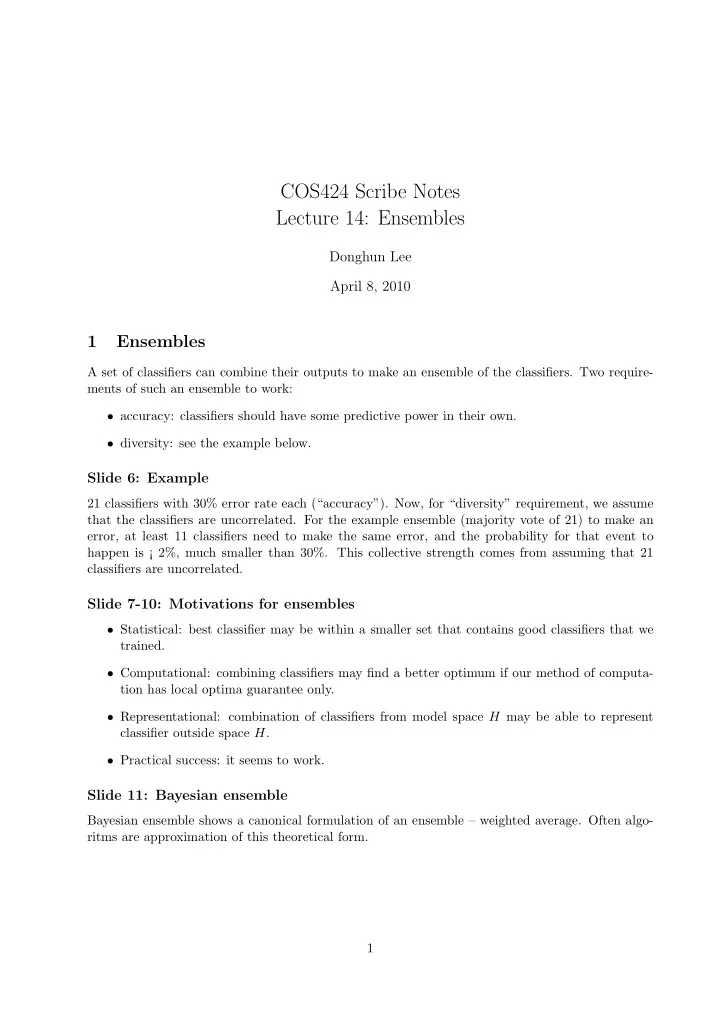
  1. COS424 Scribe Notes Lecture 14: Ensembles Donghun Lee April 8, 2010 1 Ensembles A set of classifiers can combine their outputs to make an ensemble of the classifiers. Two require- ments of such an ensemble to work: • accuracy: classifiers should have some predictive power in their own. • diversity: see the example below. Slide 6: Example 21 classifiers with 30% error rate each (“accuracy”). Now, for “diversity” requirement, we assume that the classifiers are uncorrelated. For the example ensemble (majority vote of 21) to make an error, at least 11 classifiers need to make the same error, and the probability for that event to happen is ¡ 2%, much smaller than 30%. This collective strength comes from assuming that 21 classifiers are uncorrelated. Slide 7-10: Motivations for ensembles • Statistical: best classifier may be within a smaller set that contains good classifiers that we trained. • Computational: combining classifiers may find a better optimum if our method of computa- tion has local optima guarantee only. • Representational: combination of classifiers from model space H may be able to represent classifier outside space H . • Practical success: it seems to work. Slide 11: Bayesian ensemble Bayesian ensemble shows a canonical formulation of an ensemble – weighted average. Often algo- ritms are approximation of this theoretical form. 1

  2. 2 Combining Outputs • Simple averaging works well if all classifiers are uncorrelated. Simple and effective. • Weighted averaging a priori approximates Bayesian ensemble formulation, because its weights are approximating P ( h | D ) (see slide 11) with some loss function. • Weighted averaging with trained weights requires total two validation set – one for training weights and the other to measure the performace of the ensemble itself – to avoid overfitting. • Stacked classifiers is a generalization of “Weighted averaging with trained weights” method. It also requires two validation sets. As a sidenote, needing two validation sets can be beneficial in some contests, where more than one validation sets are provided (but the examples in those sets cannot be used in the training set). 3 Constructing Ensembles An ensemble may not work if the pattern is innately too difficult for its member classifiers to learn. Also, there are situations that can be handled by constructing ensembles: • Dealing with overfitting: vary training sets with techniques like bootstrapping or bagging. (Typo on slide 19: “Bootstrap”, not Boostrap) • Dealing with noisy features: ensemble methods using feature subset selection (random forest) or preprocessing the inputs (multiband speech recognition). Both works well in practice. • Dealing with multiclass problems: To resist corruption in multiclass data class labels, encode class label data into binaries (“Error Correcting Code: ECC”), and traing a set of classifiers, where each of which will predict the bits of ECC. Because of ECC, the class labels can be reconstructed easily. 4 Boosting The motivation of Boosting technique is: an ensemble of weak classifier makes stronger classifier. An example of boosting algorithm, called Adaboost (Freund and Schapire 1995), is analyzed below. Slide 24-29: How it works Adaboost algorithm is on Slide 24. Magic terms are D t ( i ) (example i ’s weight for classifier t ) and α t (ensembling weight for classifier t ). Note that class labels are 1 or − 1, so y i h t ( x i ) = − 1 only when classifier h t makes error in predicting y i . Z t is a normalization factor. Roughly speaking, D t ( i ) is the importance weight for examples. We update this each time. If example i is correctly recognized, then D t ( i ) decreases. Otherwise, the D t ( i ) will grow. i.e. incorrectly classified examples will look bigger when calculating error rate ε t (see toy example visualization in Slides 25-28). 2

  3. Slide 30-31: Analysis There is typo in Slide 30: second line of formula, second term, inside summation sign, should be � � e − y i f T ( x i ) , not e − y i f T ( x i ). α t is the weight of ensembling. The update rule α t = 1 1 − ε t 2 log can ε t be explained from the following perspective on how Adaboost works in each round: 1. Using weighted examples D t ( i ) x i instead of raw examples x i , train classifier h t that minimizes the weighted error. 2. Update α t with a value that minimizes the weighted sum of exponential losses of all classifiers. Recall that Z t is a normalization factor (of D t +1 , precisely), and also Z t is in fact the D t -weighted sum of exponential loss from α t -weighted classifier t (see the first two lines below): � Z t = D t +1 ( i ) i � D t ( i ) e − α t y i h t ( x i ) = i D t ( i ) I ( h t ( x i ) � = y i ) e − α ·− 1 + (1 − I ( h t ( x i ) � = y i )) e − α · +1 � � � = (1) i = ε t e α t − (1 − ε t ) e − α t (2) Scribe added Equation 1 to make sure that the derivation is easier to follow. The update rule of α t is formulated to minimize Z t , i.e.: α t = arg min Z t α t ∂Z t such that = 0 ∂α t ε t e α t − (1 − ε t ) e − α t = 0 e 2 α t = 1 − ε t ε t α t = 1 2 log 1 − ε t (3) ε t Note that Equation 3 is the update rule of α t . Scribe verified that ∂ 2 Z t t > 0 with the update rule ∂α 2 α t , so it is indeed argmin, not argmax. Slide 31-32: Bounding the training error Applying this update rule to D t allows us to upper-bound the training error of the ensemble, which is ≤ � Z t (this inequality the scribe could not verify). First, we apply α t to Z t in Equation 2: � 1 − ε t � ε t Z t = ε t + (1 − ε t ) ε t 1 − ε t � � = ε t (1 − ε t ) + ε t (1 − ε t ) � = 4 ε t (1 − ε t ) � 1 − 4 γ 2 = (4) t 3

  4. where γ t = 1 2 − ε t . Since all weak learners (classifiers) are assumed to have error rate ε t lower than 1 2 , inf γ t > 0. Now, approximate bound Equation 4: � t ≤ 1 − 2 γ 2 t ≤ e − 2 γ 2 1 − 4 γ 2 (5) t We’ll use the above Inequalities 5 to bound the training error: T T T � e − 2 γ 2 t = e − 2 P T t =1 γ 2 � � � 1 − 4 γ 2 Training Error ≤ Z t = t ≤ t t =1 t =1 t =1 Since inf γ t > 0, the training error is upper-bounded by an exponentially decreasing function. This suggests the power of Adaboost to make a strong ensemble out of classifiers that are assumed to be weak learners. It also suggests the fact that it gets exponentially harder to reduce training error the same amount. Note that this training error bound is obtained 1) without specific relationship between D t (weight) and h t (choice of classifier), and 2) without specific value of α t (we used the update rule for α t that is justified from argmin-of-exponential-loss perspective). Slide 32-33: Conclusion and extension In conclusion, this shows the general applicability of Adaboost as a meta-algorithm. From algo- rithmic perspective, Boosting is a greedy optimization of exponential loss. Note that exponential loss will penalize any misclassifications (“-1”) very harshly (black line in the graph on Slide 32). Adaboost variant using log-loss (less harsh penalty) is also available. The graph on the left side of Slide 33 shows how the training error (lower) and the test error (higher) decreases versus the number of rounds. Note that the test error continues to decrease even after the training error hits 0. What happens during this period is that boosting keep decreasing the margin. From this point of view, boosting can be seen as an algorithm that increases classification P t α t yh t ( x ) margin over repeated loops, where margin is defined as on Slide 33: . The graph on the P t | α t | right side of Slide 33 is the cumulative distribution of margins, where the dotted line is from the algorithm with less rounds, and the other two are from that with more rounds. This kind of behavior (the test error keep decreasing after the training error hits 0) may be simulated by using SVM with hard margin repeatedly, where in each repetition keep increasing the margin by tweaking the weight of the examples. 4

Download Presentation
Download Policy: The content available on the website is offered to you 'AS IS' for your personal information and use only. It cannot be commercialized, licensed, or distributed on other websites without prior consent from the author. To download a presentation, simply click this link. If you encounter any difficulties during the download process, it's possible that the publisher has removed the file from their server.

Recommend


More recommend