Preliminary Simulation on Jet Breakup Experiment Using High Accuracy - PDF document

Transactions of the Korean Nuclear Society Virtual Spring Meeting July 9-10, 2020 Preliminary Simulation on Jet Breakup Experiment Using High Accuracy Kernel Correction Scheme for Smoothed Particle Hydrodynamics Hae Yoon Choi a , Eung Soo Kim a * a Department of Nuclear Engineering, Seoul National University, 1 Gwanak-ro, Gwanak-gu, Seoul, South Korea * Corresponding author: kes7741@snu.ac.kr 1. Introduction the motion of individual particles. The particles have each property and are calculated through the weight function over the neighboring particles. 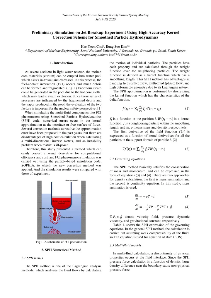The weight At severe accident in light water reactor, the molten function is defined as a kernel function which has a core materials (corium) can be erupted into water pool smoothing length. This SPH method has advantages in which exists in-vessel and ex-vessel. In this process, the handling free surface flow, multi-fluid (phase) flow, and fuel-coolant interaction (FCI) occurs and much debris high deformable geometry due to its Lagrangian nature. can be formed and fragmented. (Fig. 1) Enormous steam The SPH approximation is performed by discretizing could be generated in the pool due to the hot core melts, the kernel function which has the characteristics of the which may lead to steam explosion. Since these series of delta function. processes are influenced by the fragmented debris and the vapor produced in the pool, the evaluation of the two 𝑛 𝑘 𝑔(𝑠 𝑗 ) = ∑ 𝜍 𝑘 𝑔 𝑘 𝑋(𝑠 𝑗 − 𝑠 𝑘 ) factors is important for the nuclear safety perspective. [1] (1) 𝑘 When simulating the multi-fluid components like FCI phenomenon using Smoothed Particle Hydrodynamics 𝑔 𝑗 is a function at the position 𝑗 , 𝑋(𝑠 𝑗 − 𝑠 𝑘 ) is a kernel (SPH) code, numerical errors occur in the kernel function, 𝑘 is a neighboring particle within the smoothing approximation at the interface or free surface of flows. length, and 𝑛, 𝜍 means mass and density, respectively. Several correction methods to resolve the approximation The first derivative of the field function 𝑔(𝑠) is error have been proposed in the past years, but there are expressed as a function of kernel derivatives for all the disadvantages of high cost calculation when calculating particles in the support domain of particle 𝑗 . [2] a multi-dimensional inverse matrix, and an instability problem when matrix is ill-posed. 𝑛 𝑘 𝛼𝑔(𝑠 𝑗 ) = ∑ 𝜍 𝑘 𝑔 𝑘 𝛼𝑋(𝑠 𝑗 − 𝑠 𝑘 ) Therefore, this study presented a method which can (2) 𝑘 easily correct a kernel derivative for computational efficiency and cost, and FCI phenomenon simulation was 2.2 Governing equations carried out using the particle-based simulation code, SOPHIA, to which the new correction method was The SPH method basically satisfies the conservation applied. And the simulation results were compared with of mass and momentum, and can be expressed in the those of experiment. form of equations (3) and (4). There are two approaches for density calculation, the first is mass summation and the second is continuity equation. In this study, mass summation is used. 𝑒𝜍 𝑒𝑢 = −𝜍𝛼 ∙ 𝑣 ⃑ (3) 𝑒𝑣 ⃑ ⃑ 1 𝜈 𝑒𝑢 = − 𝜍 𝛼𝑄 + 𝜍 𝛼 2 𝑣 ⃑ + 𝑕 (4) ⃑ , 𝑄, 𝜈, 𝑕 𝑣 denote velocity field, pressure, dynamic viscosity, and gravitational constant, respectively. Table 1. shows the SPH expression of the governing equations. In the general SPH method, the calculation is carried out assuming weak compressibility of the fluid, so Tait equation is used for equation of state (EOS). Fig 1. A schematic of FCI phenomenon 2.3 Multi-fluid models 2. SPH Numerical Method In multi-fluid calculation, a discontinuity of physical properties occurs at the fluid interface. Since the SPH 2.1 SPH basics pressure force calculation is a function of density, large density difference near the boundary cause non-physical The SPH method is one of the Lagrangian analysis pressure force. methods, which analyzes the fluid flows by calculating

Transactions of the Korean Nuclear Society Virtual Spring Meeting July 9-10, 2020 Table 1. SPH Formulations uniform or the analysis area is cut off. (Fig. 2) This Mass Conservation causes not only the degradation of calculation accuracy, but also numerical instability. [3] And, the errors also Mass summation occur in the SPH approximation of the kernel derivative. 𝜍 𝑗 = ∑ 𝑛 𝑘 𝑋 In order to resolve these errors, several studies have been 𝑗𝑘 𝑘 carried out in the past, and various kernel gradient Continuity equation correction (KGC) methods have been proposed. A brief (𝑒𝜍 = 𝜍 𝑗 ∑ 𝑛 𝑘 description of KGC method is given in the next section. 𝑒𝑢) (𝑣 𝑗 ⃑⃑⃑ − 𝑣 𝑘 ⃑⃑⃑ ) ∙ 𝛼𝑋 𝑗𝑘 𝜍 𝑘 𝑗 𝑘 Momentum Conservation Pressure force (𝑒𝑣 ⃑ = ∑ − 𝑛 𝑘 𝑒𝑢) (𝑄 𝑘 + 𝑄 𝑗 )𝛼𝑋 𝑗𝑘 𝜍 𝑗 𝜍 𝑘 𝑗 𝑘 Viscous force (𝑒𝑣 ⃑ = ∑ − 4𝑛 𝑘 𝜈 𝑗 𝜈 𝑘 𝑠 ⃑⃑⃑ ∙ 𝛼𝑋 Fig 2. Truncated and non-uniform particle distribution 𝑗𝑘 𝑗𝑘 𝑒𝑢) 2 + 𝜁 2 (𝑣 𝑗 ⃑⃑⃑ − 𝑣 𝑘 ⃑⃑⃑ ) 𝜍 𝑗 𝜍 𝑘 𝜈 𝑗 + 𝜈 𝑘 𝑠 𝑗𝑘 𝑗 𝑘 3.1 Conventional kernel gradient correction Equation of State Chen (2000) proposed a corrected SPH (CSPM) from 2 𝜍 0 𝑄 = 𝑑 0 [( 𝜍 𝛿 Taylor series. CSPM provides better results than ) − 1] 𝛿 𝜍 0 conventional SPH method by solving particle deficiency problems near the boundary. [4] In the similar way, Liu et al (2006) proposed a finite particle method (FPM), Therefore, a normalized-density formulation is which is known to have greater accuracy due to its introduced to ensure stability by replacing the density simultaneous calculations on the value of the function (𝜍) with the normalized density (𝜍/𝜍 0 ) . itself and the gradient term. [5] Because the principal component direction plays a major role in the correction, 𝑛 𝑘 𝜍 ( 𝜍 0 ) = ∑ 𝜍 0,𝑘 𝑋 decoupled FPM (DFPM) which considers only the (5) 𝑘 𝑗𝑘 𝑗 principal component of FPM matrix was proposed by Zhang (2018). [6] On the other hand, Huang (2016) 𝑛 𝑘 𝑒 𝜍 𝜍 𝑗 𝑒𝑢 ( 𝜍 0 ) = − ( 𝜍 0,𝑗 ) ∑ 𝜍 𝑘 (𝑣 𝑗 ⃑⃑⃑ − 𝑣 𝑘 ⃑⃑⃑ ) ∙ 𝛼𝑋 proposed a Kernel Gradient Free (KGF) method by (6) 𝑘 𝑗𝑘 𝑗 excluding the kernel gradient itself that causes errors. [7] Table 2. shows the expression of several kernel gradient Since not only density, but also viscosity and heat correction methods. transfer coefficient are discontinuous at the interface, the The above methods improves the results in the vicinity thermal conductivity in the conduction equation is also of the interface by correcting the particle inconsistency, applied by transforming the shape as in the previous however, it is necessary to perform multi-dimensional viscous force calculation formulation. inverse matrix calculation, and in the case of ill-posed, there is a problem that the inverse matrix does not exist, 4𝑛 𝑘 𝑙 𝑗 𝑙 𝑘 𝑠 𝑗𝑘 ⃑⃑⃑⃑⃑ ∙𝛼𝑋 𝑗𝑘 𝑒ℎ 𝑗 = ∑ ( 𝑒𝑢 ) ⃑⃑⃑⃑⃑ +𝜁 2 (𝑈 𝑗 − 𝑈 𝑘 ) (7) so the calculation cost can be high and somewhat 𝑘 2 𝜍 𝑗 𝜍 𝑘 𝑙 𝑗 +𝑙 𝑘 𝑠 𝑗𝑘 inefficient. 3.2 Simplified kernel gradient correction 3. Simplified Kernel Gradient Correction Therefore, a simplified correction method was For the accurate SPH approximation, the spatial introduced to perform the calculation more efficiently. integral of the kernel function should be 1. Using the central difference approximation from Taylor series, the eqn. (10) can be derived. 𝑋 (𝑠 − 𝑠 ′ , ℎ) 𝑒𝛻 ∫ = 1 (8) 𝛻 𝜖𝑔 𝑔(𝑗 𝑆 )−𝑔(𝑗 𝑀 ) ( 𝜖𝑦 ) 𝑗 ≈ 2∆𝑦 𝑛 𝑘 ∑ 𝜍 𝑘 𝑋(𝑠 𝑗 − 𝑠 𝑘 ) = 1 (9) 𝑘 𝑛 𝑘 𝑛 𝑘 1 2∆𝑦 [∑ − ∑ = 𝜍 𝑘 𝑔 𝑘 𝑋 𝜍 𝑘 𝑔 𝑘 𝑋 ] (10) 𝑘 𝑗+∆𝑦 𝑘 𝑗−∆𝑦 The above equations are referred as unity condition, 𝑗 𝑆 , 𝑗 𝑀 indicate the position where 𝑗 particle moved very and generally satisfied inside region of the fluid for ideal slightly in the positive/negative direction. conditions. However, this condition is not satisfied near the boundary where the particle distribution is non-