Precision cosmology with 21cm intensity mapping in the - - PowerPoint PPT Presentation

Francisco ¡Villaescusa-­‑Navarro ¡-­‑-­‑-­‑ ¡INAF/INFN ¡Trieste ¡ ¡ ICTP, ¡Trieste, ¡Italy ¡– ¡13/05/2015

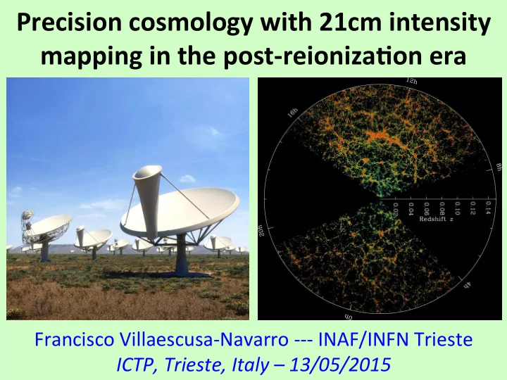
Precision ¡cosmology ¡with ¡21cm ¡intensity ¡ mapping ¡in ¡the ¡post-­‑reioniza7on ¡era ¡

MOTIVATION ¡

MOTIVATION ¡

• Study ¡the ¡Epoch ¡Of ¡Reioniza@on ¡(EOR). ¡
• Fundamental ¡to ¡understand ¡galaxy ¡forma@on/evolu@on. ¡
• Constrains ¡the ¡cosmological ¡parameters. ¡

Need ¡to ¡model ¡the ¡HI ¡ distribu@on ¡as ¡best ¡as ¡ possible ¡to ¡retrieve ¡the ¡ maximum ¡informa@on ¡ from ¡surveys ¡

P

21cm(k,z)= b21cm 2 (k,z)P m(k,z)

z ~ [2 − 5]

MODELING ¡THE ¡HI ¡DISTRIBUTION ¡

HI ¡ HII ¡ H2 ¡

Hydrogen ¡ phases ¡

NEUTRAL ¡HYDROGEN: ¡PROPERTIES ¡

1) Low ¡density ¡environments ¡ ¡ ¡ ¡ ¡ ¡ ¡ ¡ ¡ ¡ ¡(Lyman-­‑alpha ¡forest) ¡ ¡ ¡ ¡ ¡ ¡ ¡ 2) ¡High ¡density ¡environments ¡ ¡ ¡ ¡ ¡ ¡ ¡ ¡ ¡ ¡ ¡ ¡ ¡ ¡ ¡(galaxies) ¡

HII ¡

HI ¡ HII ¡

HI ¡

H2 ¡

HII ¡

HI ¡

H2 ¡

Photo-­‑ioniza;on ¡with ¡UVB ¡ HI ¡self-­‑shielding ¡ ¡ forma;on ¡of ¡molecular ¡hydrogen ¡

Hydrogen ¡phases ¡

HI ¡ HII ¡ H2 ¡

N-­‑body ¡simula7ons ¡

Photo-­‑ioniza@on ¡equilibrium ¡ HI ¡self-­‑shielding ¡ ¡ ¡ Presence ¡of ¡H2 ¡ ¡ ¡

✔ ¡ ✗ ¡ ✗ ¡

• Radia@ve ¡cooling ¡by ¡H ¡and ¡He ¡
• Hea@ng ¡by ¡uniform ¡UV ¡background ¡
• Star ¡forma@on ¡
• Feedback ¡(galac@c ¡winds) ¡

GADGET-­‑III ¡

MODELING ¡THE ¡HI ¡DISTRIBUTION ¡

Pseudo-­‑RT ¡post-­‑processing ¡

• 1. Photo-­‑ioniza@on ¡equilibrium ¡
• 2. HI ¡self-­‑shielding ¡
• 3. Presence ¡of ¡H2 ¡
• Dave ¡et ¡al. ¡2013 ¡
• Rahma; ¡et ¡al. ¡2013 ¡

MODELING ¡THE ¡HI ¡DISTRIBUTION ¡

Pseudo-­‑RT ¡post-­‑processing ¡

Method ¡ Photo-­‑ioniza7on ¡ equilibrium ¡ HI ¡self-­‑shielding ¡

Dave ¡et ¡al. ¡ 2013 ¡ ¡ Rahma@ ¡et ¡

• al. ¡2013 ¡

HI / H → ρ,T,ΓHI

Tuned ¡to ¡reproduce ¡the ¡<F> ¡of ¡the ¡Lya ¡forest ¡

NHI = 0.76m HI H ! " # $ % & mH W(r,h)dr =1017.2cm−2

rlim h

∫

HI / H → ρ,T,ΓHI

Γ phot ΓUVB = (1− f ) 1+ nH n0 # $ % & ' (

β

) * + + ,

• .

.

α1

+ f 1+ nH n0 ) * + ,

• .

α2

h

r

lim

MODELING ¡THE ¡HI ¡DISTRIBUTION ¡

Pseudo-­‑RT ¡post-­‑processing ¡

Method ¡ Presence ¡of ¡H2 ¡ ¡ ¡ ¡ Dave ¡ & ¡ Rahma@ ¡

Rmol = ΣH2 ΣHI = P / kB 1.7×104cm−3K $ % & ' ( )

0.8

fH2 =1− 0.75s 1+ 0.25s s = ln(1+ 0.6χ + 0.01χ 2) 0.6τ c χ = 0.756(1+3.1Z 0.365) τ c = Σσ d / µH

Blitz ¡& ¡Rosolowsky ¡2006 ¡ THINGS: ¡Leroy ¡et ¡al. ¡2008 ¡ ¡ Krumholz ¡& ¡Gnedin ¡2011 ¡

MODELING ¡THE ¡HI ¡DISTRIBUTION ¡

Pseudo-­‑RT ¡post-­‑processing ¡

MODELING ¡THE ¡HI ¡DISTRIBUTION ¡

bDLA(z = 2.4) =1.48

FVN, ¡Viel, ¡Da_a, ¡Choudhury, ¡2014 ¡

MODELING ¡THE ¡HI ¡DISTRIBUTION ¡

ρHI(r | M, z) M HI(M, z)

HOD/Halo ¡model ¡approach ¡ Pseudo-­‑RT ¡post-­‑processing: ¡problems ¡

• Computa@onally ¡very ¡expensive ¡
• Limited ¡to ¡rela@vely ¡small ¡volumes ¡

n(M, z) b(M, z)

Hydrodynamical ¡simula@ons ¡ Pure ¡CDM ¡simula@ons ¡ ¡ ¡ ¡ Pinocchio ¡ ¡ ¡ ¡ Halo ¡model ¡

P

L(k)

MODELING ¡THE ¡HI ¡DISTRIBUTION ¡

Semi-­‑analy@c ¡model ¡

No ¡HI ¡outside ¡halos!!! ¡

M HI(M)

Bagla ¡et ¡al. ¡2010 ¡ Barnes ¡& ¡Haehnelt ¡2014 ¡

ρHI(r)

Tuned ¡to ¡fit ¡the ¡HI ¡CDDF ¡ Find ¡DM ¡halos ¡ ¡ Compute ¡MHI(M) ¡ Distribute ¡according ¡to ¡ρHI(r) ¡

MODELING ¡THE ¡HI ¡DISTRIBUTION ¡

MODELING ¡THE ¡HI ¡DISTRIBUTION ¡

Semi-­‑analy@c ¡model ¡ Model ¡1 ¡ Model ¡2 ¡

bDLA(z = 2.4) =1.47 bDLA(z = 2.4) = 2.17

FVN, ¡Viel, ¡Da_a, ¡Choudhury, ¡2014 ¡

21 ¡cm ¡signal: ¡detectability ¡& ¡imaging ¡

SKA1-­‑MID: ¡ ¡250 ¡antennae, ¡15 ¡m ¡ SKA1 ¡LOW: ¡ ¡ 911 ¡antennae, ¡35 ¡m ¡ 100 hours FVN, ¡Viel, ¡Da_a, ¡Choudhury, ¡2014 ¡

Precision ¡cosmology ¡with ¡SKA ¡

With ¡Philip ¡Bull ¡and ¡Ma_eo ¡Viel ¡ ¡

FVN, ¡Viel, ¡Alonso, ¡Da_a, ¡Bull, ¡Santos, ¡2014 ¡

Cross-­‑correla7ng ¡21cm ¡intensity ¡maps ¡with ¡ Lyman ¡Break ¡Galaxies ¡in ¡the ¡post-­‑reioniza7on ¡era ¡

¡

Cross-­‑correla7ng ¡21cm ¡intensity ¡maps ¡with ¡ Lyman ¡Break ¡Galaxies ¡in ¡the ¡post-­‑reioniza7on ¡era ¡

¡ FVN, ¡Viel, ¡Alonso, ¡Da_a, ¡Bull, ¡Santos, ¡2014 ¡

Cross-­‑correla@ng ¡21cm ¡intensity ¡maps ¡with ¡ Lyman ¡Break ¡Galaxies ¡in ¡the ¡post-­‑reioniza@on ¡era ¡

¡

Neutral ¡hydrogen ¡

M HI(M)

HI ¡CDDF ¡

ρHI(r) ΩHI = ρHI ρc bDLA

All ¡HI ¡resides ¡in ¡halos ¡

Lyman ¡Break ¡Galaxies ¡

Bagla ¡et ¡al. ¡2010 ¡ Barnes ¡& ¡Haehnelt ¡2014 ¡

Halo ¡Occupa@on ¡Distribu@on ¡(HOD) ¡

N

M =

M M1 ! " # $ % &

α

if M > Mmin if M ≤ Mmin ( ) * * + * *

Cross-­‑correla7ng ¡21cm ¡intensity ¡maps ¡with ¡ Lyman ¡Break ¡Galaxies ¡in ¡the ¡post-­‑reioniza7on ¡era ¡

¡ FVN, ¡Viel, ¡Alonso, ¡Da_a, ¡Bull, ¡Santos, ¡2014 ¡

Cross-­‑correla7ng ¡21cm ¡intensity ¡maps ¡with ¡ Lyman ¡Break ¡Galaxies ¡in ¡the ¡post-­‑reioniza7on ¡era ¡

¡

Cross-­‑correla7ng ¡21cm ¡intensity ¡maps ¡with ¡ Lyman ¡Break ¡Galaxies ¡in ¡the ¡post-­‑reioniza7on ¡era ¡

¡ FVN, ¡Viel, ¡Alonso, ¡Da_a, ¡Bull, ¡Santos, ¡2014 ¡

WDM ¡signatures ¡on ¡the ¡21cm ¡power ¡spectrum ¡

¡

WDM ¡signatures ¡on ¡the ¡21cm ¡power ¡spectrum ¡

¡ Carucci, ¡FVN, ¡Viel ¡& ¡Lapi ¡2015 ¡

CDM 1 keV WDM total matter HI halo based HI particle based

WDM ¡signatures ¡on ¡the ¡21cm ¡power ¡spectrum ¡

¡ Carucci, ¡FVN, ¡Viel ¡& ¡Lapi ¡2015 ¡

SUMMARY ¡ ¡

• 1. Crucial ¡to ¡model ¡the ¡HI ¡distribu@on ¡from ¡the ¡theory ¡side ¡
• 2. Three ¡different ¡models ¡to ¡simulate ¡the ¡HI ¡distribu@on: ¡
• Pseudo-­‑RT ¡codes: ¡HI ¡assigned ¡to ¡gas ¡par@cles ¡individually ¡
• Semi-­‑analy@c ¡methods: ¡HI ¡assigned ¡to ¡gas ¡within ¡DM ¡halos ¡
• 3. SKA ¡will ¡detect ¡the ¡21cm ¡P(k) ¡up ¡to ¡k ¡1-­‑5 ¡h/Mpc ¡depending ¡on ¡

redshii ¡and ¡model ¡

• 4. Cross-­‑correla@ons ¡very ¡useful ¡for ¡foregrounds ¡
• 5. WDM ¡signatures ¡in ¡the ¡amplitude ¡of ¡the ¡21cm ¡power ¡spectrum ¡