Powerful tools for learning: Powerful tools for learning: Kernels - PDF document

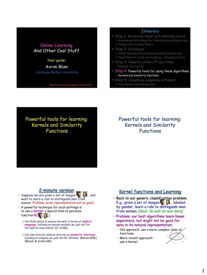
Itinerary • Stop 1: Minimizing regret and combining advice. – Randomized Wtd Majority / Multiplicative Weights alg Online Learning – Connections to game theory • Stop 2: Extensions And Other Cool Stuff – Online learning from limited feedback (bandit algs) – Algorithms for large action spaces, sleeping experts Your guide: • Stop 3: Powerful online LTF algorithms Avrim Blum – Winnow, Perceptron • Stop 4: Powerful tools for using these algorithms Carnegie Mellon University – Kernels and Similarity functions • Stop 5: Something completely different – Distributed machine learning [Machine Learning Summer School 2012] Powerful tools for learning: Powerful tools for learning: Kernels and Similarity Kernels and Similarity Functions Functions 2-minute version Kernel functions and Learning • Suppose we are given a set of images , and • Back to our generic classification problem. want to learn a rule to distinguish men from E.g., given a set of images , labeled women. Problem: pixel representation not so good. by gender, learn a rule to distinguish men • A powerful technique for such settings is from women. [Goal: do well on new data] to use a kernel : a special kind of pairwise function K ( , ) . • Problem: our best algorithms learn linear separators, but might not be good for  Can think about & analyze kernels in terms of implicit data in its natural representation. mappings , building on margin analysis we just did for Perceptron (and similar for SVMs). – Old approach: use a more complex class of - + + - functions.  Can also directly analyze directly as similarity functions , + + - - + - + – More recent approach: + + building on analysis we just did for Winnow. [Balcan- B’06] - - - [Balcan-B- Srebro’08] use a kernel. - - - - 1

Example What’s a kernel? • A kernel K is a legal def of dot-product: fn • E.g., for the case of n=2, d=2, the kernel s.t. there exists an implicit mapping  K such K(x,y) = (1 + x ¢ y) d corresponds to the mapping: that K( , )=  K ( ) ¢  K ( ). Kernel should be pos. semi- • E.g., K(x,y) = (x ¢ y + 1) d . z 2 definite (PSD) x 2 X –  K :(n-diml space) ! (n d -diml space). X X X X X X X X X • Point is: many learning algs can be written so X X O X X O O only interact with data via dot-products. X O X O X x 1 O O O X O O O z 1 – E.g., Perceptron: w = x (1) + x (2) – x (5) + x (9) . O O X O X O X O w ¢ x = (x (1) + x (2) – x (5) + x (9) ) ¢ x. X X O X X X X – If replace x ¢ y with K(x,y), it acts implicitly as if X z 3 X X X X X X data was in higher-dimensional  -space. X X Moreover, generalize well if good margin Moreover, generalize well if good margin • If data is lin. separable by But there is a little bit of a disconnect... margin  in  -space, then need • In practice, kernels constructed by viewing as a + +  sample size only Õ(1/  2 ) to get measure of similarity: K(x,y) 2 [-1,1], with some + +  extra reqts. confidence in generalization. x + - + - y - Assume |  (x)| · 1. - • But Theory talks about margins in implicit high- - dimensional  -space. K(x,y) =  (x) ¢  (y). • Can we give an explanation for desirable properties • E.g., follows directly from mistake bound we of a similarity function that doesn’t use implicit proved for Perceptron. spaces? • And even remove the PSD requirement? • Kernels found to be useful in practice for dealing with many, many different kinds of data. Goal: notion of “good similarity function” Defn satisfying (1) and (2): for a learning problem that… • Say have a learning problem P (distribution D 1. Talks in terms of more intuitive properties (no over examples labeled by unknown target f) . implicit high-diml spaces, no requirement of • Sim fn K:(x,y) ! [-1,1] is (  ,  )-good for P if at positive-semidefiniteness, etc) least a 1-  fraction of examples x satisfy: 2. If K satisfies these properties for our given problem, then has implications to learning E y~D [K(x,y)| l (y)= l (x)] ¸ E y~D [K(x,y)| l (y)  l (x)]+  3. Includes usual notion of “good kernel” (one that Average similarity to Average similarity to gap points of the same label points of opposite label induces a large margin separator in  -space). “most x are on average more similar to points y of their own type than to points y of the other type” 2

Defn satisfying (1) and (2): Defn satisfying (1) and (2): • Say have a learning problem P (distribution D • Say have a learning problem P (distribution D over examples labeled by unknown target f) . over examples labeled by unknown target f) . • Sim fn K:(x,y) ! [-1,1] is (  ,  )-good for P if at • Sim fn K:(x,y) ! [-1,1] is (  ,  )-good for P if at least a 1-  fraction of examples x satisfy: least a 1-  fraction of examples x satisfy: E y~D [K(x,y)| l (y)= l (x)] ¸ E y~D [K(x,y)| l (y)  l (x)]+  E y~D [K(x,y)| l (y)= l (x)] ¸ E y~D [K(x,y)| l (y)  l (x)]+  Average similarity to Average similarity to gap Average similarity to Average similarity to gap points of the same label points of opposite label points of the same label points of opposite label How can we use it? Note: it’s possible to satisfy this and not be PSD. How to use it How to use it At least a 1-  prob mass of x satisfy: At least a 1-  prob mass of x satisfy: E y~D [K(x,y)| l (y)= l (x)] ¸ E y~D [K(x,y)| l (y)  l (x)]+  E y~D [K(x,y)| l (y)= l (x)] ¸ E y~D [K(x,y)| l (y)  l (x)]+  • Proof: – For any given “good x”, prob of error over draw of S + ,S - at most  2 . – So, at most  chance our draw is bad on more than  fraction of “good x”. • With prob ¸ 1-  , error rate ·  +  . But not broad enough But not broad enough Avg simil to negs is ½, but to pos is only ½ ¢ 1+½ ¢ (-½) = ¼. + + + + _ _ • K(x,y)=x ¢ y has good separator but • Idea: would work if we didn’t pick y’s from top -left. doesn’t satisfy defn. (half of positives • Broaden to say: OK if 9 large region R s.t. most x are on average more similar to y 2 R of same label are more similar to negs that to typical pos) than to y 2 R of other label. (even if don’t know R in advance) 3

Broader defn… Broader defn… • Ask that exists a set R of “reasonable” y • Ask that exists a set R of “reasonable” y ( allow probabilistic ) s . t . almost all x satisfy ( allow probabilistic ) s . t . almost all x satisfy E y [K(x,y)| l (y)= l (x) , R(y)] ¸ E y [K(x,y)| l (y)  l (x) , R(y)]+  E y [K(x,y)| l (y)= l (x) , R(y)] ¸ E y [K(x,y)| l (y)  l (x) , R(y)]+  • Formally, say K is (  ,  ,  )-good if have hinge- • Formally, say K is (  ,  ,  )-good if have hinge- loss  , and Pr(R + ), Pr(R - ) ¸  . loss  , and Pr(R + ), Pr(R - ) ¸  . • Claim 1: this is a legitimate way to think • Claim 2: even if not PSD, can still use for about good (large margin) kernels: learning. – If  -good kernel then (  ,  2 ,  )-good here. – So, don’t need to have implicit -space interpretation to be useful for learning. – If  -good here and PSD then  -good kernel – But, maybe not with SVM/Perceptron directly… How to use such a sim fn? How to use such a sim fn? • Ask that exists a set R of “reasonable” y If K is (  ,  ,  )-good, then can learn to error  ’ = O() ( allow probabilistic ) s . t . almost all x satisfy with O((1/(  ’  2 )) log(n)) labeled examples. E y [K(x,y)| l (y)= l (x) , R(y)] ¸ E y [K(x,y)| l (y)  l (x) , R(y)]+  – Draw S = {y 1 ,…, y n }, n ¼ 1/(  2  ). could be unlabeled – View as “landmarks”, use to map new data: F(x) = [K(x,y 1 ), …,K( x,y n )]. – Whp, exists separator of good L 1 margin in this – Whp, exists separator of good L 1 margin in this space: w *= [0,0,1/n + ,1/n + ,0,0,0,-1/n - ,0,0] space: w *= [0,0,1/n + ,1/n + ,0,0,0,-1/n - ,0,0] – So, take new set of examples, project to this – So, take new set of examples, project to this space, and run good L 1 alg (e.g., Winnow)! space, and run good L 1 alg (e.g., Winnow)! Learning with Multiple Similarity Functions Learning with Multiple Similarity Functions • Let K 1 , …, K r be similarity functions s. t. some (unknown) • Let K 1 , …, K r be similarity functions s. t. some (unknown) convex combination of them is (  ,  )-good. convex combination of them is (  ,  )-good. Algorithm Algorithm • Draw S={y 1 ,  , y n } set of landmarks. Concatenate features. • Draw S={y 1 ,  , y n } set of landmarks. Concatenate features. F(x) = [K 1 (x,y 1 ), …,K r (x,y 1 ), …, K 1 (x,y n ),…,K r (x,y n )]. F(x) = [K 1 (x,y 1 ), …,K r (x,y 1 ), …, K 1 (x,y n ),…,K r (x,y n )]. • Run same L 1 optimization algorithm as before (or Winnow) in this Guarantee: Whp the induced distribution F(P) in R nr has a new feature space. separator of error ·  +  at L 1 margin at least Sample complexity is roughly: O((1/(  2 )) log(nr)) Only increases by log(r) factor! 4