Pipelined Computations In the pipeline technique, the problem is - - PDF document

153

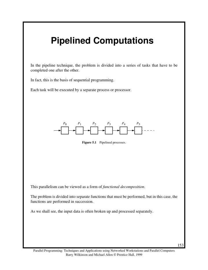
Parallel Programming: Techniques and Applications using Networked Workstations and Parallel Computers Barry Wilkinson and Michael Allen  Prentice Hall, 1999 P0 P1 P2 P3 P4 P5 Figure 5.1 Pipelined processes.

Pipelined Computations

In the pipeline technique, the problem is divided into a series of tasks that have to be completed one after the other. In fact, this is the basis of sequential programming. Each task will be executed by a separate process or processor. This parallelism can be viewed as a form of functional decomposition. The problem is divided into separate functions that must be performed, but in this case, the functions are performed in succession. As we shall see, the input data is often broken up and processed separately.

154

Parallel Programming: Techniques and Applications using Networked Workstations and Parallel Computers Barry Wilkinson and Michael Allen  Prentice Hall, 1999 sum a[0] a[1] a[2] a[3] a[4] sout sin Figure 5.2 Pipeline for an unfolded loop. sout sin sout sin sout sin sout sin a a a a a

Example Add all the elements of array a to an accumulating sum:

for (i = 0; i < n; i++) sum = sum + a[i];

The loop could be “unfolded” to yield

sum = sum + a[0]; sum = sum + a[1]; sum = sum + a[2]; sum = sum + a[3]; sum = sum + a[4]; .

One pipeline solution: Stage i performs

sout = sin + a[i];

155

Parallel Programming: Techniques and Applications using Networked Workstations and Parallel Computers Barry Wilkinson and Michael Allen  Prentice Hall, 1999 f(t) fout fin Figure 5.3 Pipeline for a frequency filter. fout fin fout fin fout fin fout fin f0 f4 f3 f2 f1 Filtered signal Signal without frequency f0 Signal without frequency f1 Signal without frequency f2 Signal without frequency f3

Example A frequency filter - The objective here is to remove specific frequencies (say the frequen- cies f0, f1, f2, f3, etc.) from a (digitized) signal, f(t). The signal could enter the pipeline from the left:

156

Parallel Programming: Techniques and Applications using Networked Workstations and Parallel Computers Barry Wilkinson and Michael Allen  Prentice Hall, 1999

Given that the problem can be divided into a series of sequential tasks, the pipelined approach can provide increased speed under the following three types of computations: 1. If more than one instance of the complete problem is to be executed 2. If a series of data items must be processed, each requiring multiple operations 3. If information to start the next process can be passed forward before the process has completed all its internal operations

157

Parallel Programming: Techniques and Applications using Networked Workstations and Parallel Computers Barry Wilkinson and Michael Allen  Prentice Hall, 1999 P0 P4 P3 P5 P2 P1

Instance 1 Instance 1 Instance 1 Instance 1 Instance 1 Instance 1 Instance 2 Instance 2 Instance 2 Instance 2 Instance 2 Instance 2 Instance 4 Instance 3 Instance 3 Instance 3 Instance 3 Instance 3 Instance 3 Instance 4 Instance 4 Instance 4 Instance 4 Instance 4 Instance 5 Instance 5 Instance 5 Instance 5 Instance 5 Instance 6 Instance 5 Instance 6 Instance 6 Instance 6 Instance 6 Instance 7 Instance 7 Instance 7 Instance 7

Time Figure 5.4 Space-time diagram of a pipeline. p − 1 m

“Type 1” Pipeline Space-Time Diagram

158

Parallel Programming: Techniques and Applications using Networked Workstations and Parallel Computers Barry Wilkinson and Michael Allen  Prentice Hall, 1999 P0 P1 P2 P3 P4 P5 P0 P1 P2 P3 P4 P5 P0 P1 P2 P3 P4 P5 P0 P1 P2 P3 P4 P5 P0 P1 P2 P3 P4 P5 Time Instance 1 Instance 2 Instance 3 Instance 0 Instance 4 Figure 5.5 Alternative space-time diagram.

159

Parallel Programming: Techniques and Applications using Networked Workstations and Parallel Computers Barry Wilkinson and Michael Allen  Prentice Hall, 1999 P0 P4 P3 P5 P2 P1 Time Figure 5.6 Pipeline processing 10 data elements. d9d8d7d6d5d4d3d2d1d0 P0 P1 P2 P3 P4 P5 (a) Pipeline structure (b) Timing diagram P8 P7 P9 P6 d0 d1 d2 d3 d4 d5 d6 d7 d8 d9 P7 P6 P8 P9 Input sequence p − 1 n d0 d1 d2 d3 d4 d5 d6 d7 d8 d9 d0 d1 d2 d3 d4 d5 d6 d7 d8 d9 d0 d1 d2 d3 d4 d5 d6 d7 d8 d9 d0 d1 d2 d3 d4 d5 d6 d7 d8 d9 d0 d1 d2 d3 d4 d5 d6 d7 d8 d9 d0 d1 d2 d3 d4 d5 d6 d7 d8 d9 d0 d1 d2 d3 d4 d5 d6 d7 d8 d0 d1 d2 d3 d4 d5 d6 d7 d0 d1 d2 d3 d4 d5 d6

“Type 2” Pipeline Space-Time Diagram

160

Parallel Programming: Techniques and Applications using Networked Workstations and Parallel Computers Barry Wilkinson and Michael Allen  Prentice Hall, 1999 Time P0 P1 P2 P3 P4 P5 (a) Processes with the same (b) Processes not with the P0 P1 P2 P3 P4 P5 Time Figure 5.7 Pipeline processing where information passes to next stage before end of process. Information transfer sufficient to start next process same execution time execution time Information passed to next stage

“Type 3” Pipeline Space-Time Diagram

161

Parallel Programming: Techniques and Applications using Networked Workstations and Parallel Computers Barry Wilkinson and Michael Allen  Prentice Hall, 1999 P0 P1 P2 P3 P4 P5 P7 P6 P8 P9 P11 P10 Processor 1 Processor 0 Processor 2 Figure 5.8 Partitioning processes onto processors.

If the number of stages is larger than the number of processors in any pipeline, a group of stages can be assigned to each processor:

162

Parallel Programming: Techniques and Applications using Networked Workstations and Parallel Computers Barry Wilkinson and Michael Allen  Prentice Hall, 1999 Host Multiprocessor computer Figure 5.9 Multiprocessor system with a line configuration.

Computing Platform for Pipelined Applications

163

Parallel Programming: Techniques and Applications using Networked Workstations and Parallel Computers Barry Wilkinson and Michael Allen  Prentice Hall, 1999 P0 P3 P2 P1 P4 Figure 5.10 Pipelined addition.

Σ

1 5

i

Σ

1

i

Σ

1 2

i

Σ

1 3

i

Σ

1 4

i

Pipeline Program Examples

Adding Numbers

The basic code for process Pi :

recv(&accumulation, Pi-1); accumulation = accumulation + number; send(&accumulation, Pi+1);

except for the first process, P0, which is

send(&number, P1);

and the last process, Pn−1, which is

recv(&number, Pn-2); accumulation = accumulation + number;

SPMD program

if (process > 0) { recv(&accumulation, Pi-1); accumulation = accumulation + number; } if (process < n-1) send(&accumulation, Pi+1);

The final result is in the last process. Instead of addition, other arithmetic operations could be done.

164

Parallel Programming: Techniques and Applications using Networked Workstations and Parallel Computers Barry Wilkinson and Michael Allen  Prentice Hall, 1999 P0 P2 P1 Pn−1 Figure 5.11 Pipelined addition numbers with a master process and ring configuration. dn−1… d2d1d0 Master process Sum Slaves

165

Parallel Programming: Techniques and Applications using Networked Workstations and Parallel Computers Barry Wilkinson and Michael Allen  Prentice Hall, 1999 P0 P2 P1 Pn−1 Figure 5.12 Pipelined addition of numbers with direct access to slave processes. Master process Sum Slaves dn−1 d0 d1 Numbers

166

Parallel Programming: Techniques and Applications using Networked Workstations and Parallel Computers Barry Wilkinson and Michael Allen  Prentice Hall, 1999

Analysis

Our first pipeline example is Type 1. We will assume that each process performs similar actions in each pipeline cycle. Then we will work out the computation and communication required in a pipeline cycle. The total execution time: ttotal = (time for one pipeline cycle)(number of cycles) ttotal = (tcomp + tcomm)(m + p − 1) where there are m instances of the problem and p pipeline stages (processes). The average time for a computation is given by

Single Instance of Problem

tcomp = 1 tcomm = 2(tstartup + tdata) ttotal = (2(tstartup + tdata) + 1)n The time complexity = Ο(n).

Multiple Instances of Problem

ttotal = (2(tstartup + tdata) + 1)(m + n − 1) ≈ 2(tstartup + tdata) + 1 That is, one pipeline cycle

Data Partitioning with Multiple Instances of Problem

tcomp = d tcomm = 2(tstartup + tdata) ttotal = (2(tstartup + tdata) + d)(m + n/d − 1) As we increase the d, the data partition, the impact of the communication diminishes. But increasing the data partition decreases the parallelism and often increases the execution time. ta ttotal m

• =

ta ttotal m

• =

167

Parallel Programming: Techniques and Applications using Networked Workstations and Parallel Computers Barry Wilkinson and Michael Allen  Prentice Hall, 1999 5 4, 3, 1, 2, 5 4, 3, 1, 2 4, 3, 1 2 5 4, 3 5 2 1 4 5 3 2 1 5 4 3 2 5 4 3 5 4 1 2 1 3 2 1 5 4 3 2 1 5 4 3 2 1 Figure 5.13 Steps in insertion sort with five numbers. P0 P2 P3 P4 P1 Time 1 2 3 4 5 6 8 7 (cycles) 9 10

Sorting Numbers

A parallel version of insertion sort. (The sequential version is akin to placing playing cards in order by moving cards over to insert a card in position ) The basic algorithm for process Pi is

recv(&number, Pi-1); if (number > x) { send(&x, Pi+1); x = number; } else send(&number, Pi+1);

With n numbers, how many the ith process is to accept is known; it is given by n − i. How many to pass onward is also known; it is given by n − i − 1 since one of the numbers re- ceived is not passed onward. Hence, a simple loop could be used.

168

Parallel Programming: Techniques and Applications using Networked Workstations and Parallel Computers Barry Wilkinson and Michael Allen  Prentice Hall, 1999 P0 P1 P2 Largest number Next largest number Series of numbers xn−1 … x1x0 Figure 5.14 Pipeline for sorting using insertion sort. xmax Compare Smaller numbers

169

Parallel Programming: Techniques and Applications using Networked Workstations and Parallel Computers Barry Wilkinson and Michael Allen  Prentice Hall, 1999 P0 P2 P1 Pn−1 Figure 5.15 Insertion sort with results returned to the master process using a bidirectional line configuration. dn−1… d2d1d0 Sorted sequence Master process

Incorporating results being returned, process i could have the form

right_procno = n - i - 1; /* no of processes to the right */ recv(&x, Pi-1); for (j = 0; j < right_procno; j++) { recv(&number, Pi-1); if (number > x) { send(&x, Pi+1); x = number; } else send(&number, Pi+1); } send(&number, Pi-1); /* send number held */ for (j = 0; j < right_procno; j++) { /* pass on other numbers */ recv(&x, Pi+1); send(&x, Pi-1); }

170

Parallel Programming: Techniques and Applications using Networked Workstations and Parallel Computers Barry Wilkinson and Michael Allen  Prentice Hall, 1999 P0 P4 P3 P2 P1 Time Figure 5.16 Insertion sort with results returned. Sorting phase Returning sorted numbers 2n − 1 n Shown for n = 5

Analysis

Sequential

Obviously a very poor sequential sorting algorithm and unsuitable except for very small n.

Parallel

Each pipeline cycle requires at least tcomp = 1 tcomm = 2(tstartup + tdata) The total execution time, ttotal, is given by ttotal = (tcomp + tcomm)(2n − 1) = (1 + 2(tstartup + tdata))(2n − 1) ts n 1 – ( ) n 2 – ( ) … 2 1 + + + + n n 1 – ( ) 2

• =

=

171

Parallel Programming: Techniques and Applications using Networked Workstations and Parallel Computers Barry Wilkinson and Michael Allen  Prentice Hall, 1999

Prime Number Generation

Sieve of Eratosthenes

A series of all integers is generated from 2. The first number, 2, is prime and kept. All multiples of this number are deleted as they cannot be prime. The process is repeated with each remaining number. The algorithm removes nonprimes, leaving only primes. Example Suppose we want the prime numbers from 2 to 20. We start with all the numbers: After considering 2, we get where the numbers with are marked as not prime and not to be considered further. After considering 3, we get Subsequent numbers are considered in a similar fashion. However, to find the primes up to n, it is only necessary to start at numbers up to . All multiples of numbers greater than will have been removed as they are also a multiple of some number equal or less than . 2, 3, 4, 5, 6, 7, 8, 9, 10, 11, 12, 13, 14, 15, 16, 17, 18, 19, 20 2, 3, 4, 5, 6, 7, 8, 9, 10, 11, 12, 13, 14, 15, 16, 17, 18, 19, 20 2, 3, 4, 5, 6, 7, 8, 9, 10, 11, 12, 13, 14, 15, 16, 17, 18, 19, 20 n n n

172

Parallel Programming: Techniques and Applications using Networked Workstations and Parallel Computers Barry Wilkinson and Michael Allen  Prentice Hall, 1999

Sequential Code

A sequential program for this problem usually employs an array with elements initialized to 1 (TRUE) and set to 0 (FALSE) when the index of the element is not a prime number. Letting the last number be n and the square root of n be sqrt_n, we might have

for (i = 2; i < n; i++) prime[i] = 1; /* Initialize array */ for (i = 2; i <= sqrt_n; i++) /* for each number */ if (prime[i] == 1) /* identified as prime */ for (j = i + i; j < n; j = j + i) /* strike out all multiples */ prime[j] = 0; /* includes already done */

The elements in the array still set to 1 identify the primes (given by the array indices). Then a simple loop accessing the array can find the primes.

Sequential time

The number of iterations striking out multiples of primes will depend upon the prime. There are n/2 − 1 multiples of 2, n/3 − 1 multiples of 3, and so on. Hence, the total sequential time is given by assuming the computation in each iteration equates to one computational step. The sequen- tial time complexity is Ο(n2). ts n 2

• 1

– n 3

• 1

– n 5

• 1

– … n n

• 1

– + + + + =

173

Parallel Programming: Techniques and Applications using Networked Workstations and Parallel Computers Barry Wilkinson and Michael Allen  Prentice Hall, 1999 P0 P1 P2 1st prime 2nd prime Series of numbers xn−1 … x1x0 Figure 5.17 Pipeline for sieve of Eratosthenes. Compare Not multiples of 3rd prime multiples number number number 1st prime number

Pipelined Implementation

The code for a process, Pi, could be based upon

recv(&x, Pi-1); /* repeat following for each number */ recv(&number, Pi-1); if ((number % x) != 0) send(&number, Pi+1);

A simple for loop is not sufficient for repeating the actions because each process will not receive the same amount of numbers and the amount is not known beforehand. A general technique for dealing with this situation in pipelines is to use a “terminator” message, which is sent at the end of the sequence. Then each process could be

recv(&x, Pi-1); for (i = 0; i < n; i++) { recv(&number, Pi-1); if (number == terminator) break; if (number % x) != 0) send(&number, Pi+1); }

174

Parallel Programming: Techniques and Applications using Networked Workstations and Parallel Computers Barry Wilkinson and Michael Allen  Prentice Hall, 1999

Solving a System of Linear Equations — Special Case

The final example is Type 3 in which the process can continue with useful work after passing on information. The objective here is to solve a system of linear equations of the so-called upper-triangular form: an−1,0x0 + an−1,1x1 + an−1,2x2 … + an−1,n−1xn−1 = bn−1 . . a2,0x0 + a2,1x1 + a2,2x2 = b2 a1,0x0 + a1,1x1 = b1 a0,0x0 = b0 where the a’s and b’s are constants and the x’s are unknowns to be found. The method used to solve for the unknowns x0, x1, x2, …, xn−1 is a simple repeated “back”

• substitution. First, the unknown x0 is found from the last equation; i.e.,

The value obtained for x0 is substituted into the next equation to obtain x1; i.e., The values obtained for x1 and x0 are substituted into the next equation to obtain x2: and so on until all the unknowns are found. Clearly, this algorithm can be implemented as a pipeline. The first pipeline stage computes x0 and passes x0 onto the second stage, which computes x1 from x0 and passes both x0 and x1 onto the next stage, which computes x2 from x0 and x1, and so on. x0 b0 a0,0

• =

x1 b1 a1,0x0 – a1,1

• =

x2 b2 a2,0x0 – a2,1x1 – a2,2

• =

175

Parallel Programming: Techniques and Applications using Networked Workstations and Parallel Computers Barry Wilkinson and Michael Allen  Prentice Hall, 1999 x0 x0 x0 x0 x1 x1 x1 x2 x2 x3 Figure 5.18 Solving an upper triangular set of linear equation using a pipeline. Compute x0 Compute x1 Compute x2 Compute x3 P0 P1 P2 P3

The ith process (0 < i < n) receives the values x0, x1, x2, …, xi-1 and computes xi from the equation xi bi ai,jx j

j = i 1 –

∑

– ai,i

• =

176

Parallel Programming: Techniques and Applications using Networked Workstations and Parallel Computers Barry Wilkinson and Michael Allen  Prentice Hall, 1999

Sequential Code

Given the constants ai,j and bk stored in arrays a[][] and b[], respectively, and the values for unknowns to be stored in an array, x[], the sequential code could be

x[0] = b[0]/a[0][0]; /* x[0] computed separately */ for (i = 1; i < n; i++) { /* for remaining unknowns */ sum = 0; for (j = 0; j < i; j++ sum = sum + a[i][j]*x[j]; x[i] = (b[i] - sum)/a[i][i]; }

177

Parallel Programming: Techniques and Applications using Networked Workstations and Parallel Computers Barry Wilkinson and Michael Allen  Prentice Hall, 1999

Parallel Code

The pseudocode of process Pi (1 < i < n) of one pipelined version could be

for (j = 0; j < i; j++) { recv(&x[j], Pi-1); send(&x[j], Pi+1); } sum = 0; for (j = 0; j < i; j++) sum = sum + a[i][j]*x[j]; x[i] = (b[i] - sum)/a[i][i]; send(&x[i], Pi+1);

(P0 simply computes x0 and passes x0 on.) Now we have additional computations to do after receiving and resending values.

178

Parallel Programming: Techniques and Applications using Networked Workstations and Parallel Computers Barry Wilkinson and Michael Allen  Prentice Hall, 1999 Time P0 P1 P2 P3 P4 P5 Figure 5.19 Pipeline processing using back substitution. Processes Final computed value First value passed onward

179

Parallel Programming: Techniques and Applications using Networked Workstations and Parallel Computers Barry Wilkinson and Michael Allen  Prentice Hall, 1999

Analysis

For this pipeline, we cannot assume that the computational effort at each pipeline stage is the same. The first process, P0, performs one divide and one send(). The ith process (0 < i < n − 1) performs i recv()s, i send()s, i multiply/add, one divide/ subtract, and a final send(), a total of 2i + 1 communication times and 2i + 2 computational steps assuming that multiply, add, divide, and subtract are each one step. The last process, Pn−1, performs n − 1 recv()s, n − 1 multiply/adds, and one divide/sub- tract, a total of n − 1 communication times and 2n − 1 computational steps.

P0 P1 P2 P3 P4 divide send(x0) ⇒ recv(x0) end send(x0) ⇒ recv(x0) multiply/add send(x0) ⇒ recv(x0) divide/subtract multiply/add send(x0) ⇒ recv(x0) send(x1) ⇒ recv(x1) multiply/add send(x1) ⇒ end send(x1) ⇒ recv(x1) multiply/add multiply/add send(x1) ⇒ recv(x1) divide/subtract multiply/add send(x1) ⇒ send(x2) ⇒ recv(x2) multiply/add end send(x2) ⇒ recv(x2) multiply/add send(x2) ⇒ divide/subtract multiply/add send(x3) ⇒ recv(x3) end send(x3) ⇒ multiply/add divide/subtract send(x4) ⇒ end Figure 5.20 Operations in back substitution pipeline. Time