Physics 2D Lecture Slides Lecture 24: Mar 1 st Vivek Sharma UCSD - - PDF document

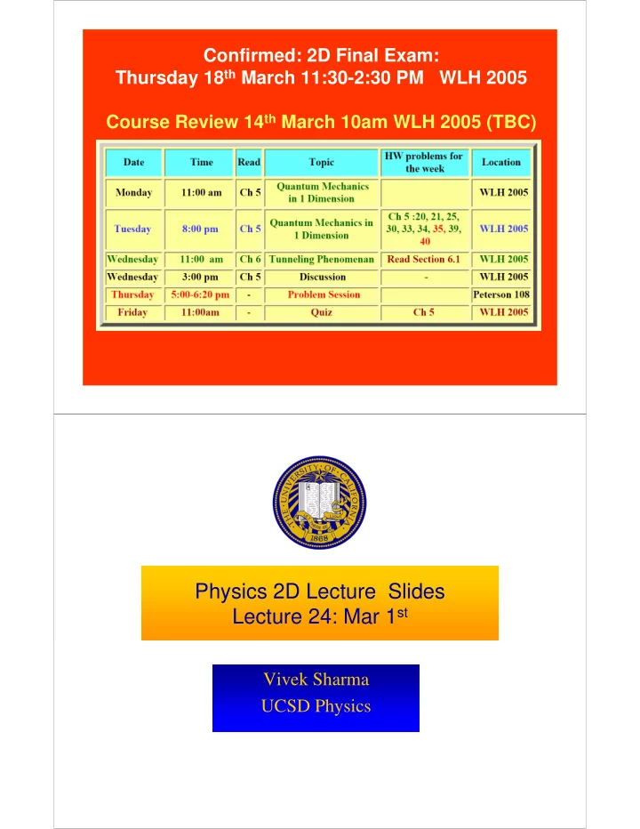
Confirmed: 2D Final Exam: Thursday 18th March 11:30-2:30 PM WLH 2005 Course Review 14th March 10am WLH 2005 (TBC)

Physics 2D Lecture Slides Lecture 24: Mar 1st

Vivek Sharma UCSD Physics

Quiz 7

5 10 15 20

1 2 3 4 5 6 7 8 9 10 11 12 13 14 15 16 17 18 19 20

Grades

Frequency

Common mistakes:

• 1. Needed to translate x x+ L/2
• 2. Difference between probability and probability amplitude !
• 3. For photon, using E = P2/2m is a very bad idea

Finite Potential Barrier

• There are no Infinite Potentials in the real world

– Imagine the cost of as battery with infinite potential diff

• Will cost infinite $ sum + not available at Radio Shack
• Imagine a realistic potential : Large U compared to KE

but not infinite

X=0 X=L U E=KE Region I Region II Region III Classical Picture : A bound particle (no escape) in 0<x<L Quantum Mechanical Picture : Use ∆E.∆t ≤ h/2π Particle can leak out of the Box of finite potential P(|x|>L) ≠0

Finite Potential Well

2 2 2 2 2 2 2 2

• ( )

( ) ( ) 2m ( ) 2 ( ) ( ) 2m(U-E) = ( ); = General Solutions : ( ) Require finiteness of ( ) ( )

x x

d x U x E x dx d x m U E x dx x x x e x Ae Be A

α α

ψ ψ ψ ψ ψ ψ α ψ α ψ ψ

+ − +

+ = ⇒ = − ⇒ ⇒ = + =

• Again, coefficients A & B come from matching conditions

at the edge of the .....x<0 (region I) walls (x =0, L) But note th .....x>L (regi at wave fn at ( ) at (x =0, L) 0 !

• n III

( ) ! )

x x

x x Ae

α α

ψ ψ

−

≠ = ( ) Further require Continuity of ( ) and These lead to rather different wave funct (why?) ions d x x dx ψ ψ

Finite Potential Well: Particle can Burrow Outside Box

Finite Potential Well: Particle can Burrow Outside Box

Particle can be outside the box but only for a time ∆t ≈ h/ ∆E ∆E = Energy particle needs to borrow to Get outside ∆E = U-E + KE The Cinderella act (of violating E Conservation cant last very long Particle must hurry back (cant be caught with its hand inside the cookie-jar)

1 Penetration Length = = 2m(U-E) If U>>E Tiny penetration If U δ α δ ⇒ → ∞ ⇒ →

• Finite Potential Well: Particle can Burrow Outside Box

1 Penetration Length = = 2m(U-E) If U>>E Tiny penetration If U δ α δ ⇒ → ∞ ⇒ →

• 2

2 2 n 2 n

n E = , 1,2,3,4... 2 ( 2 ) When E=U then solutions blow up Limits to number of bound states(E ) When E>U, particle is not bound and can get either reflected or transmitted across the potential "b n m L U π δ = + ⇒ <

• arrier"

Simple Harmonic Oscillator: Quantum and Classical

m

k

X=0 x Spring with Force Const U(x) x a b c

Stable Stable Unstable

2 2 2 2

Particle of mass m within a potential U(x) ( ) F(x)= - ( ) F(x=a) = - 0, F(x=b) = 0 , F(x=c)=0 ...But... look at the Cur 0 (stable), < 0 (uns vature: tabl ) e dU x dx dU x dx U U x x = ∂ ∂ > ∂ ∂

• 2

2

Stable Equilibrium: General Form : 1 U(x) =U(a)+ ( ) 2 Motion of a Classical Os Ball originally displaced from its equilib cillator (ideal) irium position, 1 R mo escale tion co ( ) ( nfined betw 2 e x ) en k x U x k x a a − − ⇒ =

2 2 2 2

=0 & x=A Changing A changes E E can take any value & if A 1 U(x)= ; 0, E

• Max. KE at x = 0, KE= 0 at x=

. 2 2 2 1 A 1 k m x Ang F kx kA req m E ω ω → → = ⇒ = = ± =

Quantum Picture: Harmonic Oscillator

2 2 2 2 2 2 2 2 2 2

Find the Ground state Wave Function (x) 1 Find the Ground state Energy E when U(x)= 2 1 Time Dependen

• ( )

( ) ( ) t Schrodinger Eqn: 2 ( ) 2 m 2 x x E x m x d x m dx m x x ψ ψ ψ ψ ψ ω ω ∂ + ∂ = ⇒ =

• 2

2

( ( ) 0 What (x) solves this? Two guesses about the simplest Wavefunction: 1. (x) should be symmetric about x 2. (x) 0 as x (x) + (x) should be continuous & = continu )

• s

1 u 2 m E x d dx x ψ ψ ψ ω ψ ψ ψ − = → → ∞

2

Need to find C & : What does this wavefu My nct (x) = ion & guess: PDF l C ;

• ok

like?

x

e α α ψ

−

Quantum Picture: Harmonic Oscillator

2

(x) = C

x

e α ψ

−

2

2 2

P(x) = C

x

e

α −

x C0 C2 How to Get C0 & α ?? …Try plugging in the wave-function into the time-independent Schr. Eqn.

Time Independent Sch. Eqn & The Harmonic Oscillator

2 2 2 2 2 2 2

2 2 2 2 2 2 2 2 2 2 2 2 2 2 2

Master Equation is : ( ) Since ( ) , ( 2 ) , ( ) ( 2 ) ( 2 ) [4 2 ] 1 [ ( ) 2 1 [ ] ( ) 2 2 [ ] Match t 4 ] 2 2

x x x x x x x

d x x C e C x e dx d x d x C e C x e C x e dx dx C x x e m x m m x E x x m C e E

α α α α α α α

ψ ψ α ψ α α α α α ω ψ ω ψ α

− − − − − − −

= = − − = + − ∂ = − = − ⇒ − = − ∂

• 2

2 2 2 2

he coeff of x and the Constant terms on LHS & RHS m

• r =

2 & the other match gives 2 2 = , substituing 1 E= =hf !!!!...... Planck's Oscil ( ) 2 2 1 4 2 ? We What about la s tor m m C m E ω α α ω α α ω = ⇒ ⇒

• learn about that from the Normalization cond.

SHO: Normalization Condition

2 2

1 4 2 2

(dont memorize this) Identi a= and using th | ( ) | 1 Si fying nce e identity above Hence the Complete NORMA L

m x ax

x dx C e dx e dx a m m C

ω

ω ω π ψ π

+∞ +∞ − −∞ −∞ +∞ − −∞

⎡ ⎤ ⇒ = = ⎢ ⎥ ⎣ ⎦ = =

∫ ∫ ∫

• 2

1 4 2

IZED wave function is : (x) = Ground State Wavefunction Planck's Oscillators were electrons tied by the "spring" of has energy E = h the f

m x

m e

ω

ω ψ π

−

⎡ ⎤ ⎢ ⎥ ⎣ ⎦

• mutually attractive Coulomb Force

Quantum Oscillator In Pictures

• A

+A

C0

Quantum Mechanical Prob for particle To live outside classical turning points Is finite !

• A

+A

U U(x)

( ) 0 for n=0 E KE U x = + >

Classically particle most likely to be at the turning point (velocity=0) Quantum Mechanically , particle most likely to be at x=x0 for n=0

Classical & Quantum Pictures of SHO compared

• Limits of classical vibration : Turning Points (do on

Board)

• Quantum Probability for particle outside classical turning

points P(|x|>A) =16% !!

– Do it on the board (see Example problems in book)

Excited States of The Quantum Oscillator

2 2 2

2 1 2 2 3 3 n n

( ) ( ) ; ( ) Hermite Polynomials with H (x)=1 H (x)=2x H (x)=4x 2 H ( 1 1 ( ) ( ) 2 2 n=0,1,2,3... Qu x)=8x 1 antum # H (x 2 Again )=(-1)

n x x n m x n n n n n

x C H x e H x x and d e e d E n x n hf

ω

ω ψ

− −

= + = + ∞ = = − −

• Excited States of The Quantum Oscillator

Ground State Energy >0 always

Measurement Expectation: Statistics Lesson

• Ensemble & probable outcome of a single measurement or the

average outcome of a large # of measurements

1 1 2 2 3 3 1 1 2 3 1 *

( ) .... ... ( ) For a general Fn f(x) ( ( ) ( ) ( ) ( ) ) ( )

n i i i i i i n i i i

xP x dx n x n x n x n x n x x n n n n N P x dx n f x f x N x f x x dx P x dx ψ ψ

∞ = −∞ ∞ − ∞ −∞ ∞ −∞ ∞ =

+ + + < >= = = + + + < >= =

∑ ∫ ∫ ∫ ∑ ∫

2 i 2 2

Sharpness of A Distr Scatter around average

(x ) = = ( ) ( ) = small Sharp distr. Uncertainty X = : x N x x σ σ σ σ − − → ∆

∑

Particle in the Box, n=1, <x> & ∆x ?

• 2

2 2 2 2

2 (x)= sin L 2 <x>= sin L 2 = sin , change variable = L 2 <x>= sin , L 2L <x>= d 2 sin L 1 use sin cos2 (1 cos2

• 2

) 2

L

x L x dx x d L x x dx x x L L L

π π π

π ψ π π π θ θ θ π θ π θ θ θ θ π θ θ

∞ ∞

⎛ ⎞ ⎜ ⎟ ⎝ ⎠ ⎛ ⎞ ⎜ ⎟ ⎛ ⎞ ⎜ ⎟ ⎝ ⎠ = ⎝ ⎠ ⎛ ⎞ ⎛ ⎞ ⎜ ⎟ ⎜ ⎟ ⎝ ⎠ ⎝ ⎠ ⇒ ⎡ − ⇒ ⎢ ⎣

∫ ∫ ∫ ∫ ∫

L 2 2 2 2 2 2 2 2 2 2 2 2 2 2 2

Similarly <x >= x s use ud L <x>= (same result as from graphing ( )) 2 2 in ( ) 3 2 and X= <x 0.18 3 2 4 X= 20% of L, Particle not sharply confi v=uv- ned vdu L L x dx L L L L L x L x π ψ π π π π ⎤ ⎥ ⎦ ⇒ = − ∆ > ⎛ ⎞ = ⎜ ⎟ − < > = − − = ⎠ ∆ ⎝

∫ ∫ ∫

in Box

Expectation Values & Operators: More Formally

• Observable: Any particle property that can be measured

– X,P, KE, E or some combination of them,e,g: x2 – How to calculate the probable value of these quantities for a QM state ?

• Operator: Associates an operator with each observable

– Using these Operators, one calculates the average value of that Observable – The Operator acts on the Wavefunction (Operand) & extracts info about the Observable in a straightforward way gets Expectation value for that

• bservable

* * 2

ˆ ( , ) [ ] ˆ [ ] is the operator & is the Expectation va ( , ) is the observable, [X] = x , lue [P] = [P] [K] = 2 Exam i p : m les x t d Q x t Q Q Q d dx x Q

+∞ −∞

< >= Ψ < Ψ >

∫

• 2

2 2 [E] =

• 2m

i t x ∂ = ∂ ∂ ∂

Operators Information Extractors

2 + + * *

• 2

2

ˆ [p] or p = Momentum Operator i gives the value of average mometum in the following way: ˆ [K] or K = - <p> = (x) gi [ ] ( ) = (x) i Similerly 2m : d p x dx dx dx d dx d dx ψ ψ ψ ψ

∞ ∞ ∞ ∞

⎛ ⎞ ⎜ ⎟ ⎝ ⎠

∫ ∫

• +

+ 2 2 * * 2

• +

*

• +

* *

• ( )

<K> = (x)[ ] ( ) (x) 2m Similerly <U> = (x ves the value of )[ ( )] ( ) : plug in the U(x) fn for that case an average K d <E> = (x)[ ( )] ( ) (x) E d x K x dx dx dx U x x dx K U x x dx ψ ψ ψ ψ ψ ψ ψ ψ ψ

∞ ∞ ∞ ∞ ∞ ∞ ∞ ∞ ∞

⎛ ⎞ = − ⎜ ⎟ ⎝ ⎠ + =

∫ ∫ ∫ ∫

• +

2 2 2

( ) ( ) 2m The Energy Operator [E] = i informs you of the averag Hamiltonian Operator [H] = [K] e energy +[U] d x U x dx dx t ψ

∞

⎛ ⎞ − + ⎜ ⎟ ⎝ ⎠ ∂ ∂

∫

• Plug & play form

[H] & [E] Operators

• [H] is a function of x
• [E] is a function of t …….they are really different operators
• But they produce identical results when applied to any solution of the

time-dependent Schrodinger Eq.

• [H]Ψ(x,t) = [E] Ψ(x,t)
• Think of S. Eq as an expression for Energy conservation for a

Quantum system

2 2 2

( , ) ( , ) ( , ) 2 U x t x t i x t m x t ⎡ ⎤ ∂ ∂ ⎡ ⎤ − + Ψ = Ψ ⎢ ⎥ ⎢ ⎥ ∂ ∂ ⎣ ⎦ ⎣ ⎦

Where do Operators come from ? A touchy-feely answer

i(kx-wt) i( x-wt) i( x-wt)

Consider as an example: Free Particle Wavefu 2 k = :[ ] The momentum Extractor (operator) nction (x,t) = Ae ; (x,t) (x,t) = Ae ; A , e :

p p

h p k p rewrit p i i Example p e x π λ λ Ψ ∂Ψ = ∂ = = Ψ = ⇒

• (x,t)

(x,t) = p (x,t) i So it is not unreasonable to associate [p]= with observable p i p x x Ψ ∂ ⎡ ⎤ ⇒ Ψ Ψ ⎢ ⎥ ∂ ⎣ ⎦ ∂ ⎡ ⎤ ⎢ ⎥ ∂ ⎣ ⎦

• Example : Average Momentum of particle in box
• Given the symmetry of the 1D box, we argued last time that <p> = 0

: now some inglorious math to prove it !

– Be lazy, when you can get away with a symmetry argument to solve a problem..do it & avoid the evil integration & algebra…..but be sure!

[ ]

* * 2 2 *

2 sin( )cos( ) 1 n Since sinax cosax dx = sin ...here a = 2a L sin 2 2 ( ) sin( ) & ( ) si ( n( )

n n x L x

d p p dx dx i dx n n n p x x dx i L L L L ax n p x iL n n x x x x L L L L L ψ ψ ψ ψ π π π π π π π ψ ψ

+∞ ∞ −∞ −∞ ∞ −∞ = =

⎡ ⎤ < >= = ⎢ ⎥ ⎣ ⎦ < >= ⎡ ⎤ ⇒< >= ⎢ ⎥ ⎣ = = ⎦

∫ ∫ ∫ ∫

• 2

2

Quiz 1: What is the <p> for the Quantum Oscillator in its symmetric ground st 0 since Sin (0) Sin ( ) ate Quiz 2: What is We knew THAT befor the <p> for the Qua e doing ntum Osc any i l ma la t t h

• r in it

! s nπ = = = asymmetric first excited state

But what about the <KE> of the Particle in Box ?

2 n

p 0 so what about expectation value of K= ? 2m 0 because 0; clearly not, since we showed E=KE Why ? What gives ? Because p 2 ; " " is the key! AVERAGE p =0 , particle i s moving b

n

p K p n mE L π < >= < >= < ≠ ± = ± ± >= =

• 2

2

ack & forth p <p <KE> = < > 0 not ! 2m 2 Be careful when being "lazy" Quiz: what about <KE> of a quantum Oscillator? Does similar logic apply?? m > ≠

Measurement Expectation: Statistics Lesson

• Ensemble & probable outcome of a single measurement or the

average outcome of a large # of measurements

1 1 2 2 3 3 1 1 2 3 1 *

( ) .... ... ( ) For a general Fn f(x) ( ( ) ( ) ( ) ( ) ) ( )

n i i i i i i n i i i

xP x dx n x n x n x n x n x x n n n n N P x dx n f x f x N x f x x dx P x dx ψ ψ

∞ = −∞ ∞ − ∞ −∞ ∞ −∞ ∞ =

+ + + < >= = = + + + < >= =

∑ ∫ ∫ ∫ ∑ ∫

2 i 2 2

Sharpness of A Distr Scatter around average

(x ) = = ( ) ( ) = small Sharp distr. Uncertainty X = : x N x x σ σ σ σ − − → ∆

∑

Particle in the Box, n=1, <x> & ∆x ?

• 2

2 2 2 2

2 (x)= sin L 2 <x>= sin L 2 = sin , change variable = L 2 <x>= sin , L 2L <x>= d 2 sin L 1 use sin cos2 (1 cos2

• 2

) 2

L

x L x dx x d L x x dx x x L L L

π π π

π ψ π π π θ θ θ π θ π θ θ θ θ π θ θ

∞ ∞

⎛ ⎞ ⎜ ⎟ ⎝ ⎠ ⎛ ⎞ ⎜ ⎟ ⎛ ⎞ ⎜ ⎟ ⎝ ⎠ = ⎝ ⎠ ⎛ ⎞ ⎛ ⎞ ⎜ ⎟ ⎜ ⎟ ⎝ ⎠ ⎝ ⎠ ⇒ ⎡ − ⇒ ⎢ ⎣

∫ ∫ ∫ ∫ ∫

L 2 2 2 2 2 2 2 2 2 2 2 2 2 2 2

Similarly <x >= x s use ud L <x>= (same result as from graphing ( )) 2 2 in ( ) 3 2 and X= <x 0.18 3 2 4 X= 20% of L, Particle not sharply confi v=uv- ned vdu L L x dx L L L L L x L x π ψ π π π π ⎤ ⎥ ⎦ ⇒ = − ∆ > ⎛ ⎞ = ⎜ ⎟ − < > = − − = ⎠ ∆ ⎝

∫ ∫ ∫

in Box

Schrodinger Eqn: Stationary State Form

• Recall when potential does not depend on time explicitly U(x,t)

=U(x) only…we used separation of x,t variables to simplify Ψ(x,t) = ψ(x) φ(t) & broke S. Eq. into two: one with x only and another with t only

2 2 2

• ( )

( ) ( ) ( ) 2m ( ) ( ) x U x x E x x t i E t t ψ ψ ψ φ φ ∂ + = ∂ ∂ = ∂

• How to put Humpty-Dumpty back together ? e.g to say how to

go from an expression of ψ(x)→Ψ(x,t) which describes time-evolution of the overall wave function

( , ) ( ) ( ) x t x t ψ φ Ψ =

Schrodinger Eqn: Stationary State Form [ ]

t=0

integrate both sides w.r.t. time 1 ( ) ( ) t 1 ( ) ( ) d 1 d ( ) Since ln ( ) dt ( ) dt ( ) In i ( ) , rew 1 d ( ) ( ) dt ln ( ) t ln (0) , rite as n t

• w

t t t t

and t iE dt t iE t t t E iE t i t iE dt dt f t t f t f t t E t φ φ φ φ φ φ φ φ φ φ

=

= ∂ = ∂ = − ∴ − = ∂ = = − ∂ ∂ = − − ∂ ⇒

∫ ∫ ∫

• exponentiate both sides

( ) (0) ; (0) constant= initial condition = 1 (e.g) ( ) & T (x,t)= hus where E = energy of system (x)

iEt iE i t E t

e t e t e ψ φ φ φ φ

− − −

Ψ ⇒ = = ⇒ =

• Schrodinger Eqn: Stationary State Form

* * * 2

In such cases, P(x,t) is INDEPENDENT of time. These are called "stationary" states ( , ) ( ) ( ) ( because Prob is independent of tim Examples : ) ( ) | ( Pa e rtic ) |

iE iE iE iE t t t t

P x t x e x e x x e x ψ ψ ψ ψ ψ

+ − −

= Ψ Ψ = = =

• Total energy of the system depends on the spatial orie

le in a box (why?) : Quantum Oscil ntation

• f the system : charteristic of the potential

lator situat ( i why?)

• n !