Physics 2D Lecture Slides Lecture 22: Feb 24 rd Vivek Sharma UCSD - - PDF document

physics 2d lecture slides
SMART_READER_LITE
LIVE PREVIEW

Physics 2D Lecture Slides Lecture 22: Feb 24 rd Vivek Sharma UCSD - - PDF document

Confirmed: 2D Final Exam:Thursday 18 th March 11:30-2:30 PM WLH 2005 Physics 2D Lecture Slides Lecture 22: Feb 24 rd Vivek Sharma UCSD Physics Introducing the Schrodinger Equation 2 2 ( , ) ( , ) x t x t +


slide-1
SLIDE 1

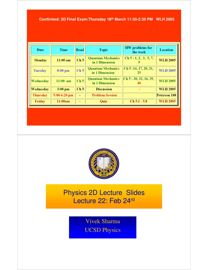
Confirmed: 2D Final Exam:Thursday 18th March 11:30-2:30 PM WLH 2005

Physics 2D Lecture Slides Lecture 22: Feb 24rd

Vivek Sharma UCSD Physics

slide-2
SLIDE 2

Introducing the Schrodinger Equation

2 2 2

( , ) ( , ) ( ) ( , ) 2 x t x t U x x t i m x t ∂ Ψ ∂Ψ − + Ψ = ∂ ∂

  • U(x) = characteristic Potential of the system
  • Different potential for different forces
  • Hence different solutions for the Diff. eqn.
  • characteristic wavefunctions for a particular U(x)

Schrodinger Wave Equation

Wavefunction which is a sol. of the Sch. Equation embodies all modern physics experienced/learnt so h E=hf, p= , . , . , quantiza tion etc Schrodinge fa r Equation is a D r: x p E t λ ψ ∆ ∆ ∆ ∆ ∼ ∼ (x,0) (x,t) Evolves the System as a function ynamical Equation much like Newton's Equation F

  • f space-time

The Schrodinger Eq. propogates the Force(potentia system forwar l d & backward = a ) m ψ ψ

→ →

  • in time:

(x, t) = (x,0) Where does it come from ?? ..."First Principles"..no real derivation exists

t

d t dt ψ ψ δ ψ δ

=

⎡ ⎤ ± ⎢ ⎥ ⎣ ⎦

slide-3
SLIDE 3

Time Independent Sch. Equation

( )

2 2 i(kx 2

  • Sometimes (depending on the character of the Potential U(x,t))

The Wave function is factorizable: can be broken up ( , ) ( , ) ( ) ( , ) 2 x,t ( ) : Plane Wave (x,t ( )=e ) Exa x t x t U x x t i m x t x mple t ψ φ ∂ Ψ ∂Ψ − + Ψ = ∂ ∂ Ψ = Ψ

  • t)

i(kx)

  • i( t)

2 2 2 2 2 2

  • ( )

( ) ( ). ( ) ( ) ( ) ( ) 2m

  • 1

( ) 1 In suc ( ) . ( ) 2m ( ) h cases, use seperation of variables to get : Divide Throughout by (x,t e e L )= HS ( ( x) ( t) s ) i x t t U x x t i x x t x t U x i x x t t

ω ω

ψ φ φ ψ φ ψ ψ φ φ ψ φ ψ ∂ ∂ + = ∂ ∂ ∂ Ψ ⇒ ∂ = ∂ + = ∂

  • a function of x; RHS is fn of t

x and t are independent variables, hence : RHS = LHS = Constant = E ⇒

Factorization Condition For Wave Function Leads to:

2 2 2

  • ( )

( ) ( ) ( ) 2m ( ) ( ) x U x x E x x t i E t t ψ ψ ψ φ φ ∂ + = ∂ ∂ = ∂

  • ikx
  • i t

ikx

What is the Constant E ? How to Interpret it ? Back to a Free particle : (x,t)= Ae e , (x)= Ae U(x,t) = 0 Plug it into the Time Independent Schrodinger Equation (TISE)

ω

ψ Ψ ⇒

2 2 2 2 2 (

  • i t

2 2 ) ( ) 2

(NR Energy) 2 2 Stationary states of the free particle: (x,t)= (x)e ( , ) ( ) Probability is static in time t, character of wave function ( ) depends on 2

ikx ikx

k p E m m x d Ae E t A dx x e m

ω

ψ ψ − = = = Ψ ⇒ = = ⇒ Ψ +

  • ( )

x ψ

slide-4
SLIDE 4

Schrodinger Eqn: Stationary State Form

  • Recall when potential does not depend on time explicitly

– U(x,t) =U(x) only…we used separation of x,t variables to simplify

  • Ψ(x,t) = ψ(x) φ(t)
  • broke S. Eq. into two: one with x only and another with t only

2 2 2

  • ( )

( ) ( ) ( ) 2m ( ) ( ) x U x x E x x t i E t t ψ ψ ψ φ φ ∂ + = ∂ ∂ = ∂

  • How to put Humpty-Dumpty back together ? e.g to say how to

go from an expression of ψ(x)→Ψ(x,t) which describes time-evolution of the overall wave function

( , ) ( ) ( ) x t x t ψ φ Ψ =

Schrodinger Eqn: Stationary State Form [ ]

t=0

integrate both sides w.r.t. time 1 ( ) ( ) t 1 ( ) ( ) d 1 d ( ) Since ln ( ) dt ( ) dt ( ) In i ( ) , rew 1 d ( ) ( ) dt ln ( ) t ln (0) , rite as n t

  • w

t t t t

and t iE dt t iE t t t E iE t i t iE dt dt f t t f t f t t E t φ φ φ φ φ φ φ φ φ φ

=

= ∂ = ∂ = − ∴ − = ∂ = = − ∂ ∂ = − − ∂ ⇒

∫ ∫ ∫

  • exponentiate both sides

( ) (0) ; (0) constant= initial condition = 1 (e.g) ( ) & T (x,t)= hus where E = energy of system (x)

iEt iE i t E t

e t e t e ψ φ φ φ φ

− − −

Ψ ⇒ = = ⇒ =

slide-5
SLIDE 5

A More Interesting Potential : Particle In a Box

U(x,t) = ; x 0, x L U(x,t) = 0 ; 0 < X < Write the Form of Potential: Infinite Wall L ∞ ≤ ≥

  • Classical Picture:
  • Particle dances back and forth
  • Constant speed, const KE
  • Average <P> = 0
  • No restriction on energy value
  • E=K+U = K+0
  • Particle can not exist outside box
  • Can’t get out because needs to borrow

infinite energy to overcome potential of wall

U(x)

What happens when the joker is subatomic in size ?? Example of a Particle Inside a Box With Infinite Potential

(a) Electron placed between 2 set of electrodes C & grids G experiences no force in the region between grids, which are held at Ground Potential However in the regions between each C & G is a repelling electric field whose strength depends on the magnitude of V (b) If V is small, then electron’s potential energy vs x has low sloping “walls” (c) If V is large, the “walls”become very high & steep becoming infinitely high for V→∞ (d) The straight infinite walls are an approximation of such a situation

U=∞

U(x)

U=∞

slide-6
SLIDE 6

Ψ(x) for Particle Inside 1D Box with Infinite Potential Walls

2 2 2 2 2 2 2 2 2 2 2

Inside the box, no force U=0 or constant (same thing) ( ) ( ) ; ( ) ( ) fig

  • ( )

( ) ( ) ure out 2m what (x) solves this diff e 2 q. In General the solu d x x E d x k x dx d x k x dx x dx mE k

  • r

ψ ψ ψ ψ ψ ψ ψ ψ ⇒ ⇒ ⇒ = − + = ⇐ + = =

  • A

t p io pl n is y BO ( ) UNDA R (A,B are constants) Need to figure out values of A, B : How to do that ? We said ( ) must be continuous everywhe Y Conditions on the Physical Wav re So efunction x A sinkx B coskx x ψ ψ = + match the wavefunction just outside box to the wavefunction value just inside the box & A Sin kL = 0 At x = 0 ( 0) At x = L ( ) ( 0) 0 (Continuity condition at x =0) & ( ) x x L x B x L ψ ψ ψ ψ ⇒ ∴ ⇒ = = ⇒ = = = = ⇒ = = =

2 2 2 n 2

(Continuity condition at x =L) n kL = n k = , 1,2,3,... L So what does this say about Energy E ? : n E = Quantized (not Continuous)! 2 n mL π π π ⇒ ⇒ = ∞

  • X=0

Why can’t the particle exist Outside the box ? E Conservation ∞ ∞ X=L

Quantized Energy levels of Particle in a Box

slide-7
SLIDE 7

What About the Wave Function Normalization ?

n We will call n Quantum Number , just like in Bohr's Hydrogen atom W The particle's Energy and Wavefu hat about the wave functions cor nct res ion a pondi re determi ng to each ned by a

  • f these

nu e mb g er ner →

n L * 2 2 2 n 2 n

y states? sin( ) sin( ) for 0<x < L = 0 for Normalized Condition : 1 x 0, x L Use 2Sin 1 2 2 2 1 1 c = ( )

  • s(

2

L

n x dx A S n x A kx A L Cos A in L π ψ θ π ψ θ ψ = = ≥ ≥ = − = − =

∫ ∫

n 2

) and since cos = sin 2 1 2 So 2 2 sin( ) sin ...What does this look ) l ( ike?

L

n x kx L L L n x L A L A L π θ π θ ψ = ⎛ ⎞ ⎜ ⎟ ⎝ ⎠ = ⇒ = =

∫ ∫

Wave Functions : Shapes Depend on Quantum # n

Wave Function

Probability P(x): Where the particle likely to be

Zero Prob

slide-8
SLIDE 8

Where in The World is Carmen San Diego?

  • We can only guess the probability
  • f finding the particle somewhere

in x

– For n=1 (ground state) particle most likely at x = L/2 – For n=2 (first excited state) particle most likely at L/4, 3L/4

  • Prob. Vanishes at x = L/2

& L

– How does the particle get from just before x=L/2 to just after? » QUIT thinking this way, particles don’t have trajectories » Just probabilities

  • f being

somewhere

Classically, where is particle most likely to be ? Equal prob. of being anywhere inside the Box NOT SO says Quantum Mechanics!

Remember Sesame Street ?

This particle in the box is brought to you by the letter

Its the Big Boss Quantum Number

slide-9
SLIDE 9

How to Calculate the QM prob of Finding Particle in Some region in Space

3 3 3 4 4 4 2 2 1 L L L 4 4 4 3 /4 /4

Consider n =1 state of the particle L 3 Ask : What is P ( )? 4 4 2 2 1 2 P = sin . (1 cos ) 2 1 2 1 1 2 3 2 sin sin . sin . 2 2 2 2 4 4 1

L L L L L

L x x x dx dx dx L L L L L L x L L P L L L L P π π ψ π π π π π ≤ ≤ ⎛ ⎞ = = − ⎜ ⎟ ⎝ ⎠ ⎡ ⎤ ⎡ ⎤ ⎛ ⎞ = − = − − ⎜ ⎟ ⎢ ⎥ ⎢ ⎥ = ⎣ ⎦ ⎣ ⎦ ⎝ ⎠

∫ ∫ ∫

Classically 50% (equal prob over half the box size) Substantial difference between Class 1 ( 1 1) 0.818 8 ical & Quantu 1. m predictio 8 n 2 s % 2π − − − ⇒ = ⇒ ⇒

When The Classical & Quantum Pictures Merge: n→∞

But one issue is irreconcilable: Quantum Mechanically the particle can not have E = 0 This is a consequence of the Uncertainty Principle The particle moves around with KE inversely proportional to the Length Of the 1D Box

slide-10
SLIDE 10

Finite Potential Barrier

  • There are no Infinite Potentials in the real world

– Imagine the cost of as battery with infinite potential diff

  • Will cost infinite $ sum + not available at Radio Shack
  • Imagine a realistic potential : Large U compared to KE

but not infinite

X=0 X=L U E=KE Region I Region II Region III Classical Picture : A bound particle (no escape) in 0<x<L Quantum Mechanical Picture : Use ∆E.∆t ≤ h/2π Particle can leak out of the Box of finite potential P(|x|>L) ≠0

Finite Potential Well

2 2 2 2 2 2 2 2

  • ( )

( ) ( ) 2m ( ) 2 ( ) ( ) 2m(U-E) = ( ); = General Solutions : ( ) Require finiteness of ( ) ( )

x x

d x U x E x dx d x m U E x dx x x x e x Ae Be A

α α

ψ ψ ψ ψ ψ ψ α ψ α ψ ψ

+ − +

+ = ⇒ = − ⇒ ⇒ = + =

  • Again, coefficients A & B come from matching conditions

at the edge of the .....x<0 (region I) walls (x =0, L) But note th .....x>L (regi at wave fn at ( ) at (x =0, L) 0 !

  • n III

( ) ! )

x x

x x Ae

α α

ψ ψ

≠ = ( ) Further require Continuity of ( ) and These lead to rather different wave funct (why?) ions d x x dx ψ ψ

slide-11
SLIDE 11

Finite Potential Well: Particle can Burrow Outside Box Finite Potential Well: Particle can Burrow Outside Box

Particle can be outside the box but only for a time ∆t ≈ h/ ∆E ∆E = Energy particle needs to borrow to Get outside ∆E = U-E + KE The Cinderella act (of violating E Conservation cant last very long Particle must hurry back (cant be caught with its hand inside the cookie-jar)

1 Penetration Length = = 2m(U-E) If U>>E Tiny penetration If U δ α δ ⇒ → ∞ ⇒ →

slide-12
SLIDE 12

Finite Potential Well: Particle can Burrow Outside Box 1 Penetration Length = = 2m(U-E) If U>>E Tiny penetration If U δ α δ ⇒ → ∞ ⇒ →

  • 2

2 2 n 2 n

n E = , 1,2,3,4... 2 ( 2 ) When E=U then solutions blow up Limits to number of bound states(E ) When E>U, particle is not bound and can get either reflected or transmitted across the potential "b n m L U π δ = + ⇒ <

  • arrier"

Simple Harmonic Oscillator: Quantum and Classical

m

k

X=0 x Spring with Force Const

slide-13
SLIDE 13

U(x) x a b c

Stable Stable Unstable

2 2 2 2

Particle of mass m within a potential U(x) ( ) F(x)= - ( ) F(x=a) = - 0, F(x=b) = 0 , F(x=c)=0 ...But... look at the Cur 0 (stable), < 0 (uns vature: tabl ) e dU x dx dU x dx U U x x = ∂ ∂ > ∂ ∂

  • 2

2

Stable Equilibrium: General Form : 1 U(x) =U(a)+ ( ) 2 Motion of a Classical Os Ball originally displaced from its equilib cillator (ideal) irium position, 1 R mo escale tion co ( ) ( nfined betw 2 e x ) en k x U x k x a a − − ⇒ =

2 2 2 2

=0 & x=A Changing A changes E E can take any value & if A 1 U(x)= ; 0, E

  • Max. KE at x = 0, KE= 0 at x=

. 2 2 2 1 A 1 k m x Ang F kx kA req m E ω ω → → = ⇒ = = ± =

Quantum Picture: Harmonic Oscillator

2 2 2 2 2 2 2 2 2 2

Find the Ground state Wave Function (x) 1 Find the Ground state Energy E when U(x)= 2 1 Time Dependen

  • ( )

( ) ( ) t Schrodinger Eqn: 2 ( ) 2 m 2 x x E x m x d x m dx m x x ψ ψ ψ ψ ψ ω ω ∂ + ∂ = ⇒ =

  • 2

2

( ( ) 0 What (x) solves this? Two guesses about the simplest Wavefunction: 1. (x) should be symmetric about x 2. (x) 0 as x (x) + (x) should be continuous & = continu )

  • s

1 u 2 m E x d dx x ψ ψ ψ ω ψ ψ ψ − = → → ∞

2

Need to find C & : What does this wavefu My nct (x) = ion & guess: PDF l C ;

  • ok

like?

x

e α α ψ

slide-14
SLIDE 14

Quantum Picture: Harmonic Oscillator

2

(x) = C

x

e α ψ

2

2 2

P(x) = C

x

e

α −

x C0 C2 How to Get C0 & α ?? …Try plugging in the wave-function into the time-independent Schr. Eqn.