Phylogenetic Methods Multiple Sequence Alignment Pairwise distance - PDF document

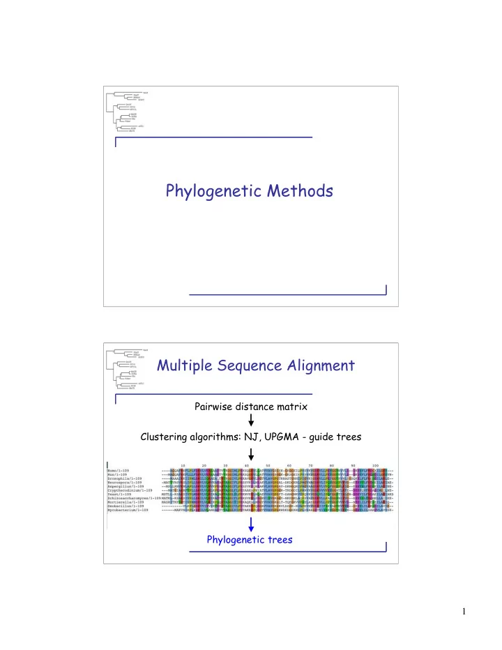
Phylogenetic Methods Multiple Sequence Alignment Pairwise distance matrix Clustering algorithms: NJ, UPGMA - guide trees Phylogenetic trees 1

Nucleotide vs. amino acid sequences for phylogenies 1) Nucleotides: - Synonymous vs. nonsynonymous substitutions - Transitions vs. transversions - Coding vs. non-coding sequences - Can analyze pseudogenes 2) Amino acids: - Distances can be very large for nucleotides - 20 characters, greater “phylogenetic signal” Today: A) Rooting phylogenetic trees B) Number of phylogenetic trees C) Tree building (character, distance) D) Testing the robustness of the tree E) Testing alternative tree topologies F) Influenza 2

Inferring evolutionary relationships requires rooting the tree B C To root a tree, imagine that the tree is made of string. Root D Unrooted tree Grab the string at the A root and tug on it until the ends of the string A B C D (the taxa) fall opposite the root: Rooted tree Root There are two major ways to root trees: By outgroup: pick outgroup that is not too tart, not too sweet outgroup A By midpoint or distance: d (A,D) = 10 + 3 + 5 = 18 Midpoint = 18 / 2 = 9 on longest path; need to 10 C be sure evolutionary rates 3 2 are same for all taxa B 2 D 5 3

The number of possible trees grows quickly # OTUs Unrooted trees Rooted trees 2 1 1 3 1 3 4 3 15 5 15 105 10 2,027,025 34,459,425 15 7.91 x 10 12 2.13 x 10 14 20 2.2 x 10 20 8.2 x 10 21 50 3.0 x 10 74 2.8 x 10 76 n (2n - 5)! / 2 n-2 (n-3)! (2n - 3)! / 2 n-2 (n-2)! There are ~10 79 protons in the universe Computational methods for finding optimal trees Exhaustive algorithms: Evaluates all possible trees, choosing the one with the best score. Heuristic algorithms: Approximate methods that attempt to find the optimal tree for the method of choice, but cannot guarantee to do so. 4

How do we build a phylogenetic tree? 1) Distance-based methods: - Transform the aligned sequences into pairwise distances - Use the distance matrix during tree building ( UPGMA, Neighbor joining, etc. ) - Decisions: how to deal with gaps? correction for multiple substitutions? How do we build a phylogenetic tree? 2) Character-based methods: - Examine aligned sequences, pick informative sites - Build tree that requires smallest number of changes ( Maximum parsimony ) - Or that has highest likelihood of producing data based on a sequence evolution model ( Maximum likelihood ) 5

Maximum parsimony methodology “ IT IS VAIN TO DO WITH MORE WHAT CAN BE DONE WITH FEWER” OR Principle of parsimony OR …smallest number of evolutionary changes… The ‘most-parsimonious’ tree is the one that requires the fewest number of evolutionary events ( e.g., nucleotide or amino acid substitutions) to explain the sequences observed in the taxa. Maximum parsimony methodology Step 1: Identify informative sites Sites with at least two different characters at the site, each of which is represented in at least two of the sequences Site Seq. 1 2 3 4 5 6 7 8 9 1 A A G A G T T C A 2 A G C C G T T C T 3 A G A T A T C C A 4 A G A G A T C C T 6

Maximum parsimony methodology Step 1: Identify informative sites Sites with at least two different characters at the site, each of which is represented in at least two of the sequences Site Seq. 1 2 3 4 5 6 7 8 9 1 A A G A G T T C A 2 A G C C G T T C T 3 A G A T A T C C A 4 A G A G A T C C T Sites where all trees require the same number of changes are not informative Tree I Tree II Tree III 1 3 1 2 1 2 G A G C G C G A A A A A C A A A A A 2 4 3 4 4 3 Site = changes Seq. 1 2 3 4 5 6 7 8 9 1 A A G A G T T C A 2 A G C C G T T C T 3 A G A T A T C C A 4 A G A G A T C C T 7

MP analyzes sites at which one substitution model requires fewer changes Tree I Tree II Tree III 1 3 1 2 1 2 G A G G G G G A A A A A G A A A A A 2 4 3 4 4 3 Site = changes Seq. 1 2 3 4 5 6 7 8 9 1 A A G A G T T C A 2 A G C C G T T C T 3 A G A T A T C C A 4 A G A G A T C C T MP analyzes sites at which one substitution model requires fewer changes Tree I Tree II Tree III 1 3 1 2 1 2 T C T T T T T C C C C C T C C C C C 2 4 3 4 4 3 Site = changes Seq. 1 2 3 4 5 6 7 8 9 1 A A G A G T T C A 2 A G C C G T T C T 3 A G A T A T C C A 4 A G A G A T C C T 8

MP analyzes sites at which one substitution model requires fewer changes Tree I Tree II Tree III 1 3 1 2 1 2 A A A T A T T T A T T T T T A T T A 2 4 3 4 4 3 Site = changes Seq. 1 2 3 4 5 6 7 8 9 1 A A G A G T T C A 2 A G C C G T T C T 3 A G A T A T C C A 4 A G A G A T C C T Maximum parsimony methodology Step 2: Calculate minimum number of substitutions at each informative site Step 3: Sum number of changes at each informative site for each possible tree The tree(s) with the least number of total changes is/are the most parsimonious tree(s) # ∆ s @ site Tree I 5 7 9 ∑ 1 3 Tree I 1 1 2 4 Tree II 2 2 1 5 2 4 Tree III 2 2 2 6 9

Maximum parsimony computations Up to ~10 OTUs: can do exhaustive search - Start with 3 taxa in a tree, add one taxon at a time - Look at all possible trees, select best tree 10-20 OTUs: start being selective - Determine a reasonably good threshold tree length - Pursue only those trees shorter than a threshold >20 OTUs: heuristic search - educated guesses - Draw initial tree with fast algorithm - Search for shorter trees by examining only trees with similar topology; pruning and regrafting Bootstrapping is used to evaluate the robustness of phylogenetic trees 1) Start with original dataset and original tree 2) Randomly re-sample with replacement to obtain alignment of equal size (pseudo-sample) 3) Build tree with re-sampled data, repeat 500-1000x 4) Determine frequency with which each clade in original tree is observed in pseudo-trees 10

Bootstrapping a phylogenetic tree 1 2 3 4 5 6 7 8 9 10 11 12 % time the same nodes A were recovered B C D Resample with replacement 2 6 1 2 4 9 7 5 3 11 1 12 A Build tree with pseudosample B C D Bootstrapping a phylogenetic tree 1 2 3 4 5 6 7 8 9 10 11 12 % time the same nodes A were recovered B C D Resample with replacement 7 7 6 3 5 2 6 8 5 10 7 7 A Build tree with pseudosample B C D 11

How are bootstrapping values interpreted? Measures how strongly the “phylogenetic signal” is distributed through the multiple sequence alignment Values > 70% are considered to support clade designations (estimated p < 0.05) Assumes samples are reasonably representative of larger population Which of two “good” trees are better? outgroup outgroup How is this tree? ? Different methods for distance, MP, and ML trees 12

Influenza virus • ssRNA genome, ~13,588 bases • Genome in 8 segments, 10-11 genes Influenza virus genes Genome Segment size segment (bases) Gene(s) Gene function 1 2341 PB2 Transcriptase: cap binding 2 2341 PB1 Transcriptase: elongation; PB1-F2 Induces apoptosis 3 2233 PA Transcriptase: protease activity 4 1778 HA Hemagglutinin: host cell recognition 5 1565 NP Nucleoprotein: RNA binding; transcriptase complex; vRNA transport 6 1413 NA Neuraminidase: release of virus 7 1027 M1 Matrix protein: major component of virion M2 Integral membrane protein - ion channel 8 890 NS1 Non-structural: RNA transport, splicing, translation. Anti-interferon. NS2 Non-structural: nucleus and cytoplasm, vRNA export (NEP) 13

Influenza nomenclature • Subtype nomenclature based on HA and NA genes • 16 Hemagglutinins, 9 Neuraminidases • Human: H: 1,2,3 ; N: 1,2; Birds: all combinations Influenza virus can change rapidly • High mutation rate (antigenic drift) • Reassortment (antigenic shift) 1 2 3 4 5 Two different viruses 6 7 1 infect same cell 8 2 3 4 5 6 7 1 8 2 3 4 Can produce 5 6 hybrid viruses 7 8 14

Reassortment can produce pandemic influenza viruses • 1957 Asian flu: H2N2, 3 avian flu segments, 5 human flu segments • 1968 Hong Kong flu: H3N2, 2 avian flu segments, 6 human flu segments • Reassortment in pigs - susceptible to avian, human, and swine flus 1918 influenza pandemic • Highly virulent flu virus (“Spanish flu”) • Estimated deaths: 50-100 million worldwide (of 1.8 billion) • Many people died within a few days from acute pneumonia • Many fatalities were young and healthy people • Lowered average U.S. life expectancy by 10 years 15

Spread of the 1918 flu in the U.S. 1918 influenza questions • Where did the 1918 flu come from? • Why was the 1918 flu so pathogenic? • Is it possible for a 1918-like pandemic to happen again? 16

Avian flu H5N1 • Has jumped to humans (> 250 people infected) • Very little immunity in humans: mortality rate ~60% • Can have similar pathology to 1918 virus • How close is avian flu to being able to efficiently infect humans and spread from human to human? 17