csce 471 871 lecture 5 building phylogenetic trees
play

CSCE 471/871 Lecture 5: Building Phylogenetic Trees Building trees - PDF document

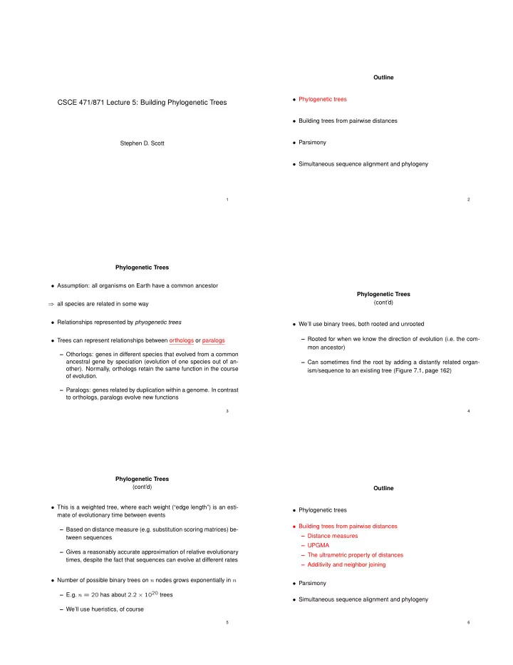
Outline Phylogenetic trees CSCE 471/871 Lecture 5: Building Phylogenetic Trees Building trees from pairwise distances Parsimony Stephen D. Scott Simultaneous sequence alignment and phylogeny 1 2 Phylogenetic Trees


  1. Outline • Phylogenetic trees CSCE 471/871 Lecture 5: Building Phylogenetic Trees • Building trees from pairwise distances • Parsimony Stephen D. Scott • Simultaneous sequence alignment and phylogeny 1 2 Phylogenetic Trees • Assumption: all organisms on Earth have a common ancestor Phylogenetic Trees (cont’d) ) all species are related in some way • Relationships represented by phyogenetic trees • We’ll use binary trees, both rooted and unrooted – Rooted for when we know the direction of evolution (i.e. the com- • Trees can represent relationships between orthologs or paralogs mon ancestor) – Othorlogs: genes in different species that evolved from a common ancestral gene by speciation (evolution of one species out of an- – Can sometimes find the root by adding a distantly related organ- other). Normally, orthologs retain the same function in the course ism/sequence to an existing tree (Figure 7.1, page 162) of evolution. – Paralogs: genes related by duplication within a genome. In contrast to orthologs, paralogs evolve new functions 3 4 Phylogenetic Trees (cont’d) Outline • This is a weighted tree, where each weight (“edge length”) is an esti- • Phylogenetic trees mate of evolutionary time between events • Building trees from pairwise distances – Based on distance measure (e.g. substitution scoring matrices) be- – Distance measures tween sequences – UPGMA – Gives a reasonably accurate approximation of relative evolutionary – The ultrametric property of distances times, despite the fact that sequences can evolve at different rates – Additivity and neighbor joining • Number of possible binary trees on n nodes grows exponentially in n • Parsimony – E.g. n = 20 has about 2 . 2 ⇥ 10 20 trees • Simultaneous sequence alignment and phylogeny – We’ll use hueristics, of course 5 6

  2. Building Trees from Pairwise Distances Building Trees from Pairwise Distances UPGMA (cont’d) UPGMA 1. 8 i , assign seq x i to cluster C i and give it its own leaf, with height 0 • Start with some distance measure between sequences 2. While there are more than two clusters – E.g., Jukes-Cantor: d ij = � 0 . 75 log(1 � 4 f ij / 3) , where f ij is (a) Find minimum d ij in distance matrix fraction of residues that differ between sequences x i and x j when (b) Add to the clustering cluster C k = C i [ C j and delete C i and C j pairwise aligned (c) For each cluster C ` 62 { C k , C i , C j } 1 • UPGMA (unweighted pair group method average) algorithm X d k ` = d pq | C k | | C ` | – One of a family of hierarchical clustering algorithms p 2 C k ,q 2 C ` – Basic overall idea of this algorithmic family: Find minimum inter- [Shortcut: Eq. (7.2)] cluster distance d ij in current distance matrix, merge clusters i and (d) Add to the tree node k with children i and j , with height d ij / 2 j , then update distance matrix 3. When only C i and C j remain, place root at height d ij / 2 – Differences among algorithms lie in matrix update – For phylogenetic trees, also add edge lengths Example: Fig 7.4, page 168 7 8 Building Trees from Pairwise Distances Building Trees from Pairwise Distances Neighbor Joining UPGMA (cont’d) • If the ultrametric property doesn’t hold, can still recover original tree if additivity holds • If the rate of evolution is the same at all points in original (target) phy- – I.e. if, in the original tree, the distance between any pair of leaves logenetic tree, then UPGMA will recover the correct tree = the sum of the lengths of the edges of the path connecting them – This occurs iff length of all paths from root to leaves are equal in • If additivity holds, then neighbor joining finds the original tree terms of evolutionary time – First, find a pair of neighboring leaves i and j , assign them parent k , then replace i and j with k , where for all other leaves m , • If this is not the case, then UPGMA may find incorrect topology (Fig. 7.5, d km = ( d im + d jm � d ij ) / 2 p. 170) – But it does NOT work to simply choose the pair ( i, j ) with minimum d ij (See Fig. 7.7, p. 171) – Instead, choose ( i, j ) minimizing D ij = d ij � ( r i + r j ) , where L • Can avoid this if distances satisfy ultrametric condition: for any three is current set of “leaves” and sequences x i , x j , x k , the distances d ij , d jk , d ik are either all equal, or 1 r i = X d ik two are equal and one is smaller | L | � 2 k 2 L 9 10 Outline Building Trees from Pairwise Distances Neighbor Joining (cont’d) • Phylogenetic trees 1. Initialize L = T = set of leaves • Building trees from pairwise distances 2. While | L | > 2 (a) Choose i and j minimizing D ij • Parsimony (b) Define new node k and set d km = ( d im + d jm � d ij ) / 2 for all m 2 L – Weighted parsimony (c) Add k to T with edges of lengths d ik = ( d ij + r i � r j ) / 2 and – Score computation d jk = d ij � d ik (d) Update L = { k } [ L \ { i, j } – Branch and bound 3. Add final, length- d ij edge between final nodes i and j • Simultaneous sequence alignment and phylogeny 11 12

  3. Parsimony Parsimony Scoring a Tree • Very widely used approach for tree building • Scores a tree based on the cost of substitutions in going from a node 1. Initialize k = 2 n � 1 (index of the root node) to its child ) will assign hypothetical ancestral sequences to internal nodes 2. Recursively compute S k ( a ) for all a in the alphabet: • Example, page 174 (unit costs) (a) If k is a leaf, set S k ( a ) = 0 for a = x k u and S k ( a ) = 1 otherwise • Generally consists of two components ) a must match u th symbol in sequence 1. Computing cost of tree T over n aligned sequences 2. Searching through the space of possible trees for min-cost one (b) Else S k ( a ) = min b ( S i ( b ) + S ( a, b )) + min b ( S j ( b ) + S ( a, b )) , where i and j are k ’s children • Treat each site independently of the others, so for a length- m align- ment, run the scoring algorithm on each of the m sites separately 3. Return min a S 2 n � 1 ( a ) as minimum cost of tree • Let S ( a, b ) be cost of substituting b for a • Scoring site (tree) u 2 { 1 , . . . , m } , let S k ( a ) be the minimal cost for Can recover ancestral residues by tracking where min comes from in the assignment of symbol (residue) a to node k recurisve step 13 14 Parsimony Searching for a Tree Outline • Not practical to enumerate the entire set of possible trees and score them all • Phylogenetic trees • Will use branch and bound to speed it up (though no guarantee of an • Building trees from pairwise distances efficient algorithm) – When incrementally building a tree, adding edges will never de- • Parsimony crease its cost – Thus if a tree’s cost already exceeds the final cost of the best tree • Simultaneous sequence alignment and phylogeny so far, we can discard it – Hein’s affine cost algorithm • Algorithm: systematically grow existing tree by adding edges, stopping expansion if current tree’s cost exceeds final cost of best tree so far 15 16 Simultaneous sequence alignment and phylogeny Simultaneous sequence alignment and phylogeny Hein’s Affine Cost Algorithm Hein’s Affine Cost Algorithm Finding Set of Sequences that Best Align with Leaves • Similar to parsimony in that, given a topology, it infers ancestral se- • GOAL: Given sequences x and y , find set of sequences such that quences for each such sequence z , S ( x, z ) + S ( z, y ) = S ( x, y ) (for either mismatch scores or weighted scores) • But this algorithm uses an affine gap penalty model (separate penal- • Use dynamic programming to handle affine gap penalties, avoiding ties for opening and extending gaps) alternating gaps: – V M ( i, j ) = min cost aligning x 1 ...i to y 1 ...j with x i aligned to y j • First, it ascends the tree from the leaves, determining the set of se- quences that best align with leaf sequences V M ( i, j ) min { V M ( i � 1 , j � 1) , V X ( i � 1 , j � 1) , = V Y ( i � 1 , j � 1) } + S ( x i , y j ) – Represents such a set of sequences as a digraph – V X ( i, j ) = min cost aligning x 1 ...i to y 1 ...j with x i aligned to gap • Then it works its way up toward the root, at each step inferring the set V X ( i, j ) = min { V M ( i � 1 , j ) + d, V X ( i � 1 , j ) + e } of sequences that best align with the child graphs – V Y ( i, j ) = min cost aligning x 1 ...i to y 1 ...j with y j aligned to gap • Finally, it descends from the root to the leaves, fixing the specific an- V Y ( i, j ) = min { V M ( i, j � 1) + d, V Y ( i, j � 1) + e } cestral sequences 17 18

Download Presentation
Download Policy: The content available on the website is offered to you 'AS IS' for your personal information and use only. It cannot be commercialized, licensed, or distributed on other websites without prior consent from the author. To download a presentation, simply click this link. If you encounter any difficulties during the download process, it's possible that the publisher has removed the file from their server.

Recommend


More recommend