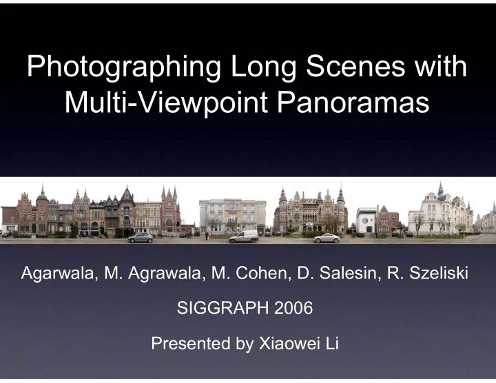
Photographing Long Scenes with Multi-Viewpoint Panoramas Agarwala, - - PowerPoint PPT Presentation

Photographing Long Scenes with Multi-Viewpoint Panoramas

Agarwala, M. Agrawala, M. Cohen, D. Salesin, R. Szeliski SIGGRAPH 2006 Presented by Xiaowei Li

Keywords in the Title

• Multi-Viewpoint

Single-Viewpoint

• Panoramas
• Long Scenes

Single-Viewpoint

One “camera”, one shot; Unique perspective rule on one picture.

Single-Viewpoint

Ancient artists knew this.

Multi-Viewpoint

• Just many Single Viewpoint ...
• Inside one picture, different portion has

different perspective rules.

• In this paper, many single-viewpoint

photos rendered in one picture naturally.

Panoramas

• Strip Panoramas
• Single-Viewpoint Panoramas
• Multi-Viewpoint Panoramas

Panoramas

• Strip Panoramas
• also known as “Slit Scan”.
• pushbroom cameras/ 1D camera
• satellite images.
• also can obtained by sampling normal 2D

image sequences [Zheng2003, Levin2005]. Vertical pixel strips from each image in the sequence.

Panoramas

• Strip Panoramas by sampling image

sequences [Zheng 2003]

Panoramas

• Strip Panoramas by sampling image

sequences Orthographic projection along horizontal axis; Perspective projection along vertical axis. Main Problem Different aspect ratio at different depth

• >closer squashed; further stretched.

Panoramas

• Strip Panoramas by sampling image

sequences

Main Problem Different aspect ratio at different depth

• >closer squashed; further stretched.

many adaptive or interactive method to choose different width for pixel strip for

• bjects at different depth. however, still
• pen problem.

Panoramas

• Strip Panoramas by sampling image

sequences Main Problem Different aspect ratio at different depth

• >closer squashed; further stretched.

Panoramas

• Strip Panoramas by sampling image

sequences by different slit method [Roman 04, thesis 06]

Panoramas

• Strip Panoramas by sampling image

sequences Other problems

• Lose local perspective effects

horizontally.

• video cameras on cars: in general,

lower resolution; shake, blurring; motion restricted as camera moving on a flat plane (ground).

Panoramas

• Single-Viewpoint Panoramas
• most normal panoramas: wide angle cameras.
• using images from pure rotating cameras

[Szeliski 97]

• using approximate rotating cameras [Lowe’s

autostitch] Hard for long scene ...

Panoramas

• Multi-Viewpoint Panoramas
• by using multiple images
• single cross-slits
• multiple cross-slits
• This paper, totally different scheme.

Panoramas

• Multi-Viewpoint Panoramas

Why?

• A photograph with a wider field of view would

cause distortion towards the edges of the image.

• Far enough away from the scene we will lose the

depth cues of the scene.

• Such panoramas can be used to visually convey

directions through a city,

• or to visualize how proposed architecture would

appear within the context of an existing street.

Long Scene Panorama Applications

• Street View - really long [Roman 04,

thesis 06]...

Long Scene Panorama Applications

• Ancient Street View by royal artist Zhang Zeduan

800-900 years ago

Long Scene Panorama Applications

• Virtual Earth/Google Earth
• really long in 2 directions

This work

• Multi-viewpoint panorama long roughly

planar scenes (facades of the buildings along a city street).

• Significantly different from previous strip

panoramas.

• After a small user interaction, the system

will automatically compute a panorama with a MRF optimization.

• Users may exert additional control over

the appearance of the result.

Quick Example

Quick Example

Quick Example

Quick Example

Previous Strip Panoramas

• Assumptions
• Orthographic projection along the horizontal axis
• Perspective projection along the vertical axis
• Shortcomings
• Only objects at a certain depth from the camera

plane can be shown with a correct aspect ratio.

• Further objects appear horizontally stretched.
• Closer objects appear squashed.

What is a Good Multi-Viewpoint Panorama

• Each object in the scene is rendered

from a viewpoint roughly in front of it.

• The panoramas are composed of large

regions of linear perspective.

• Local perspective effects are evident.
• The seams between these perspective

regions do not draw attention.

System Overview

Text

A Key Observation

• Images projected onto the picture

surface from their original 3D viewpoints will agree in areas depicting scene geometry lying on the dominant plane.

Data Capture

• Handheld camera
• walk along street and take picture every meter.
• manually control exposure.
• Fisheye lens for some scenes.
• Cover more scene content in one picture to

avoid frequent “viewpoint transition”.

Preprocessing

• Image Correction
• For photos from fisheye lens, use

PtLens to remove the radial distortion. Then treat them as normal images.

Preprocessing

• Recovering of the projection matrices of

each camera using the structure-from- motion system

• The one in Photo Tourism, which is

now open source.

• Pair-wise matching on SIFT features

enforces strong constraints for

• ptimization.

Camera 3D position

Preprocessing

• SfM result
• Each image’s projection matrix and 3D

point cloud for the scene strucure.

Picture not from this project!!

Preprocessing

• Compensation of exposure variation
• Brightness scale factor ki

i for each image Ii

• For pixels that depict the same geometry, asserting

that ki*Ii = kj*Ij for Ii , Ij

• Each SIFT point match gives us three linear

constraints of these form.

• Picture surface?

A virtual 3D surface upon which the panorama will be formed.

• It should be roughly aligned to the

dominant plane of the scene. why? Good property 1.

Picture Surface Selection

Blue curves

Picture Surface Selection

X- axis Z- axis

• Two steps: 1 Find world coordinate.

2 Draw curve in xz plane.

• The system offers an automatic and an

interactive approaches for choosing the coordinate system:

• automatic approach -- PCA; largest variation is

x-axis, least is y-axis. Because it’s facade scene.

• interactive approach -- The cross product from two

selected vectors along the y and x-axis forms the z-axis; the cross product of z and y forms the new x-axis.

Picture Surface Selection

Picture Surface Selection

• The user is asked to draw a polyline into

the plan view (xz slice).

• The system sweeps the polyline up and

down the y−axis.

• Directly draw manually
• Interactively draw -- select clusters of scene points;

remove outliers; fit a third-degree polynomial z (x ) as a function of their x−coordinates; swept up this surface and down the y-axis.

Red: recovered camera trajectory. Blue: user drawn polyline Data Videos directly interactively

Sampling the Picture Surface

• The system samples the picture surface to form a

regular 2D grid. This 2D grid will map to make the final panorama image space.

• S (i , j ) refers the 3D location of the (i,j) sample.

Sampling the Picture Surface

i j ... ... This surface will form the final panorama after projected to 2D it’s a 3D surface. so (i,j) --> S(i, j)

• Project all S(i, j) with each image’s projection

matrix.

• Each sample S (i , j ) forms one pixel, if its

projection is located inside that image.

• so there will be black holes and edges highly
• distorted. (white board)‏

Sampling the Picture Surface

Sampling the Picture Surface

One Source Image Its Sampled Image (after a circular crop)

Sampling the Picture Surface

• They also call this process as projecting

source images onto picture surface.

• Project all source images to picture surface by

“sampling picture surface”.

• Produce an average image with all these

projected images.

Average Image

... average

Average Image

• After all source images get projected to

3D surface and sampled. Average Average with un-warping and cropping

Street not straight, due to Sfm drifting Corrected by un-warping

Average Image

Recall: image areas on dominant plane will be consistent after reprojected to picture surface.

Viewpoint Selection

• We have now a series of n images Ii of

equivalent dimension.

• Image Ii represents the i’th viewpoint.
• It’s necessary to choose one source

image Ii for each pixel p = (px , py)

Again, pixel labelling problem

Objective Function

• The MRF optimization computes a

labeling L(p), where L(p) = i if pixel p of the panorama is assigned color Ii (p).

• The objective function for choosing the

viewpoint has three terms.

First Term

• The first term reflects the property that

an object in the scene should be imaged from a viewpoint roughly in front of it.

• Assuming the cameras have roughly the

same distance from the picture surface.

• It’s possible to find pixel pi whose

corresponding 3D Sample S (pi) is closest to camera position Ci .

• So, if pixel p chooses its color from Ii,

formulate this heuristic as:

Second Term

• The second term encourages transitions

between different regions of linear perspective to be natural and seamless. For all neighboring pixels.

Third Term

• The third term encourages the panorama

to resemble the average image in areas where the scene geometry intersects the picture surface.

• Recall: the key observation

Also, it’s used for many other variance, like motion blur, occlusion

• A vector median filter is used to compute

across the three color channels for a robust mean value.

• The median absolute deviation (MAD) is

calculated as median L2 distance from the median color.

Third Term

Third Term

• Assuming that image color channels vary

from 0 to 255, it’s possible to define the cost function:

Complete Cost Function

• Pixels in Image Ii to which the i’th

camera does not project are set as null -- > the black holes.

• L(p) = i is not possible if Ii (p) = null.
• Higher values for α encourage pixels

from more straight-on views at the expense of more noticeable seams.

• Lower values of both α and β are more

likely to remove objects off of the dominant plane.

• 100 β

0 25 i t ll

Solve it as a MRF Optimization

• The panorama is computed at a lower

resolution so that the MRF optimization can be computed in reasonable time.

• Using the hierarchical approach a

higher-resolution is recreated.

• The final panorama is composited in the

gradient domain to smooth the seams.

Interactive Refinement

• View selection
• A certain viewpoint should be used for a

certain region of the composite.

• Seam suppression
• The user can indicate objects in a scene

across which seams should never placed.

• Inpainting (Similar to image completion)

The user can draw strokes to indicate areas that should be filled with zero gradients during gradient-domain composition (to remove for example power lines)‏

Seam Suppression

• The MRF Optimization try to route seams

around objects that lie off the dominant plane.

• However, such objects don’t always exist.

Shortened car in the automatic panorama User strokes in

• ne source

image

Seam Suppression

• Propagate the stroked pixels
• assume the strokes are drawn on 3D

planes.

• transfer the pixels to other source

images by a homography (2D/2D relationship)

Seam Suppression

• Constraints on these stroked pixels (on

all images): for each pixel q adjacent to p that L(p) = i, if and only if L(q) = i.

• -> keep that whole region as much as

possible.

Full Example 1

Data

Projected Source

Average Image

Seams Found

Red lines are where the labeling changes-->Seams

Result

Automatically computed

Full Example 2

Data

Projected Source

Initial Result

Automatically computed

User Strokes

User wants to maintain perspective in these areas.

Seams

No seams pass the area covered by strokes.

Final Result

Before After