Periodic Lorentz gas One moving particle bounces off a periodic array - PowerPoint PPT Presentation

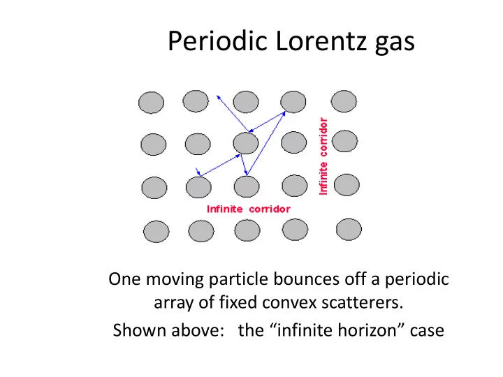
Periodic Lorentz gas One moving particle bounces off a periodic array of fixed convex scatterers. Shown above: the “infinite horizon” case

“ Finite horizon” case: Larger scatterers blocking the particle from all sides. No infinite corridors.

Symbols and notation q(t) position of the particle at time t v(t) velocity of the particle at time t q n position of the particle at n th collision v n velocity of the particle at n th collision

No external forces, finite horizon: q ( t ) ~ N ( 0,D 0 t ) as t → ∞ (asymptotically normal) D 0 is diffusion matrix ( integral of autocorrelations ) D 0 = ∫ R < v ( t ) v ( 0 )> μ dt ^ q n ~ N ( 0,D 0 n ) as n → ∞ (asymptotically normal) ^ D 0 is diffusion matrix ( infinite sum of autocorrelations ) ^ D 0 = Σ < dq n dq 0 > ν ^ D 0 = τ D 0 where τ is the mean free path Sinai & Bunimovich 1981

No external forces, infinite horizon: q ( t ) ~ N ( 0,D 1 t log t ) as t → ∞ (superdiffusive) D 1 is superdiffusion matrix Chernov & Dolgopyat 2009 ^ q n ~ N ( 0,D 1 n log n ) as n → ∞ (superdiffusive) ^ D 1 is superdiffusion matrix ( finite sum of parameters of corridors ) Szász & Varjú 2007 ^ D 1 = τ D 1 where τ is the mean free path

Lorentz gas with a constant external force Particle (“electron”) is subject to an external (“electric”) field E = ( ε ,0) directed horizontally ε >0 is small

Lorentz gas with external field: Equations of motion dq/dt = v dv/dt = E Total energy (kinetic + potential) is preserved: ½ v 2 ‐ ε x = const Thus when the particle is driven by the field and x(t) grows, then v(t) has to grow, too: v 2 = O( x ) This is unrealistic for an actual electrical current. Electrons are expected to travel at a linear rate, i.e. < x > = Jt , where J represents the current

Lorentz gas with a thermostat Electrons move subject to a force and thermostat : dq/dt = v dv/dt = E ‐ <E,v>v Gaussian thermostat (Moran & Hoover 1987)

Lorentz gas with a thermostat Electrons move subject to a force and thermostat: dq/dt = v dv/dt = E ‐ < E,v > v Now <v,v>=1 at all times, because < v , dv/dt > = 0 In other words, the kinetic energy is kept constant. The extra term prevents the electrons from speeding ( heating up ) or slowing down ( cooling down ). It keeps the temperature fixed. Hence its name: thermostat .

Gaussian thermostat, finite horizon Then q ( t ) ~ J 0 t + N ( 0, D 0 ( ε ) t ) (drift + diffusion) The electrical current J 0 satisfies J 0 = σ 0 E + o( ε ) (Ohm’s law) recall: ε = | E | Electrical conductivity σ 0 satisfies σ 0 = ½ D 0 (Einstein relation) D 0 is again the diffusion matrix (for the field ‐ free process) D 0 ( ε ) = D 0 + o(1) as ε → 0 Note: the current J 0 is not always parallel to the field E (this is known as Hall effect in physics) Chernov, Eyink, Lebowitz, Sinai 1993 and Chernov, Dolgopyat 2009

Gaussian thermostat, infinite horizon Assume: the field E is not parallel to any infinite corridor Then q ( t ) ~ J 1 t + N ( 0, D 1 ( ε ) t ) (drift + diffusion) The electrical current J 1 does not satisfy Ohm’s law: J 1 = σ 1 E |log ε |+ O( ε ) recall: ε = | E | Superconductivity coefficient σ 1 satisfies σ 1 = ½ D 1 (Einstein relation still holds) D 1 is again the diffusion matrix (for the field ‐ free process) D 1 ( ε ) = D 1 |log ε | + O(1) Chernov, Dolgopyat 2009

Back to Lorentz gas with external field No thermostat is imposed anymore. Questions: Describe asymptotic behavior of the position and velocity of the particle as time t → ∞ .

Equivalent to Galton board An upright board with a periodic array of fixed pegs on which balls are rolling down bouncing off the pegs Introduced by Sir Francis Galton (1822 ‐ 1911) Resembles a modern pinball machine

Galton board dynamics Galton board is an upright plane with fixed

Difficulties: • Particle accelerates as it moves away • Phase space is not compact, invariant measure is infinite • Initial distribution is concentrated in a compact domain (say, 0 ≤ x , y ≤ 1) • Images of the initial measure escape to infinity • Dynamics is inhomogeneous in time and space (speed increases, trajectory straightens)

For the Lorentz gas/Galton board with a constant external field and finite horizon Conjectures in physics literature 1979 ‐ 2008 (based on heuristic and empirical studies): Position x ( t ) ~ t 2/3 Velocity v ( t ) ~ t 1/3 Note: the electron travels at a slow (sublinear) rate. The reason is: backscattering (“Fermi acceleration”)

Chernov & Dolgopyat 2009: Average position x(t) does grow as t 2/3 Average velocity v(t) does grow as t 1/3 Rescaled position t ‐ 2/3 x(t) has a limit distribution Rescaled velocity t ‐ 1/3 v(t) has a limit distribution Rescaled position converges to an Itô diffusion process satisfying certain Stochastic Differential Equations

Chernov & Dolgopyat 2009: The limit stochastic process is recurrent (comes back to x =0 infinitely many times). The original trajectory x ( t ) is recurrent, too: the particle’s coordinate returns to its initial value x ( 0 ) infinitely many times with probability one. A surprising fact, but intuitively follows from the invariance of an infinite measure

Lorentz gas with external field and infinite horizon This remains an open problem. We (C&D) are currently working on it. Our conjectures: Position x ( t ) ~ ( t log t ) 2/3 Velocity v ( t ) ~ ( t log t ) 1/3

The finite horizon Galton board was studied via approximating it by the Lorentz gas with Gaussian thermostat. Both are ε− perturbations of the field ‐ free (billiard) dynamics, and they are ε 2 − close to each other. So knowing one, we can effectively study the other.

For the infinite horizon Galton board this approach fails. Here is the reason: The trajectories with and without Gaussian thermostat are actually ( ε 2 t 3 ) − close to each other, where t is the time between collisions. In finite horizon, t =O(1), so we have ε 2 − closeness In infinite horizon, t =O( ε −1/2 ), so we only have ε 1/2 − closeness, which is very poor.

So we introduce a new thermostatted model : The particle moves under the constant field (along a parabola, with its speed growing) between collisions, but its energy is reset at each collision. We call this thermostatted walls . By the way, this is a more physically sensible thermostat (Gaussian thermostat was criticized by many as unrealistic). But it causes unforeseen and peculiar complications: the dynamics ceases to be invertible . • Some phases points may have more than one preimage ( indeterminate past ). • Some phase points may have no preimages at all ( no past ).

To visualize the situation: Let F : T → T be a hyperbolic automorphism of a 2 ‐ torus. Let T = M 1 Ú ∙∙∙ Ú M k be a partition of T into domains with piecewise smooth boundaries. Let G : T → T be a map that is smooth on each M i and its restriction to M i is a C 2 ‐ perturbation of the identity map on M i . Then the composition F O G is a map that has strong expansion and contraction, but the images of M i may overlap and/or may leave uncovered gaps in T . Such maps were studied recently by operator technique Baladi & Gouëzel 2009 and 2010

We (C&D) use standard pairs, Growth Lemma, and Coupling Lemma to: Prove the existence and uniqueness of a physically observable (SRB ‐ like) measure. Establish exponential decay of correlations and limit theorems. We only work with general unstable, i.e., expanding curves (we do not need unstable manifolds) and only iterate them forward.

Final results for the Lorentz gas with thermostatted walls: All the limit theorems about the drift, (super)diffusion, (super)conductivity, etc., previously proven for the Gaussian thermostat are now proven for the thermostatted walls. Both in finite and infinite horizon. Chernov & Dolgopyat 2010