[PDF] - Page 1 Inverse Problems - Examples Inverse Problems - Theory PDF Document

SLIDE 1

Page 1

Computational Photography Ivo Ihrke, Summer 2007

Inverse Problems

Ivo Ihrke

Computational Photography Ivo Ihrke, Summer 2007

Outline

Theory

example 1D deconvolution Fourier method Algebraic method

discretization
matrix properties
regularization
solution methods
Computed Tomography (CT)

Radon transform Filtered Back-Projection natural phenomena glass objects

Computational Photography Ivo Ihrke, Summer 2007

Inverse Problem - Definition

forward problem

given a mathematical model M and its

parameters m, compute (predict) observations o inverse problem

given observations o and a mathematical model

M, compute the model's parameters

= M(m)

m = M −(o)

Computational Photography Ivo Ihrke, Summer 2007

Inverse Problems - Examples

forward problem – volume rendering

given voxel data and image formation model,

compute a view of the object

m are the volume coefficents, c is

the ray that determines the pixel's value o (observation)

=
c m(c(s))ds

Computational Photography Ivo Ihrke, Summer 2007

Inverse Problems - Examples

inverse problem – CT

given the pixel values o, the ray geometry c and

the image formation model, compute the volume densities m

invert n is a noise component we will later see how to do this

3D

=
c

m(c(s))ds + n

Computational Photography Ivo Ihrke, Summer 2007

Inverse Problems - Examples

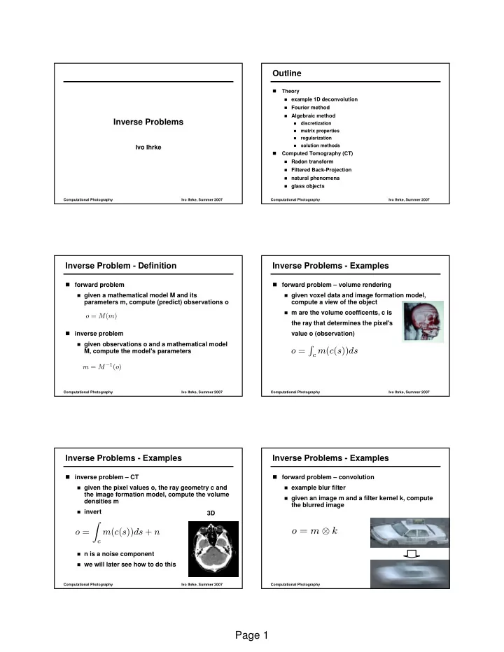
forward problem – convolution

example blur filter given an image m and a filter kernel k, compute

the blurred image

= m ⊗ k

SLIDE 2

Page 2

Computational Photography Ivo Ihrke, Summer 2007

Inverse Problems - Examples

inverse problem – deconvolution

example blur filter given a blurred image o and a filter kernel k,

compute the sharp image

need to invert n is again noise

= m ⊗ k + n

Computational Photography Ivo Ihrke, Summer 2007

Inverse Problems - Theory

deconvolution in Fourier space convolution theorem ( F is the Fourier transform ): deconvolution: problems

division by zero Gibbs phenomenon

(ringing artifacts)

= m ⊗ k ⇔ F(o) = F(m) F(k)

F(m) = F(o) F(k)

Computational Photography Ivo Ihrke, Summer 2007

A One-Dimensional Example – Deconvolution Spectral

most common: is a low pass filter

, the inverse filter, is a high pass filter
amplifies noise and numerical errors

F(k)

F k

Computational Photography Ivo Ihrke, Summer 2007

A One-Dimensional Example – Deconvolution Spectral

reconstruction is noisy even if data is perfect !

Computational Photography Ivo Ihrke, Summer 2007

A One-Dimensional Example – Deconvolution Spectral

spectral view of signal, filter and inverse filter

Computational Photography Ivo Ihrke, Summer 2007

A One-Dimensional Example - Deconvolution Spectral

solution: restrict frequency response of high pass filter (clamping)

G =

F k

, if

|F k| < γ

γ F k

|F k|

, else M = O G

SLIDE 3

Page 3

Computational Photography Ivo Ihrke, Summer 2007

A One-Dimensional Example - Deconvolution Spectral

reconstruction with clamped inverse filter

Computational Photography Ivo Ihrke, Summer 2007

A One-Dimensional Example- Deconvolution Algebraic

alternative: algebraic reconstruction convolution discretization: linear combination of basis functions

(x) =

∞

−∞

m(t)k(x − t)dt m(t) =

N

i

miφi(t)

Computational Photography Ivo Ihrke, Summer 2007

A One-Dimensional Example – Deconvolution Algebraic

discretization:

bservations are

linear combinations

f convolved basis

functions

linear system with

unknowns

ften over-

determined, i.e. more observations o than degrees of freedom ( basis functions )

=

m ⊗ k = ∞

−∞

m(t)k(x − t)dt ≈ ∞

−∞ N

i

miφi(t)k(x − t)dt =

N

i

mi ∞

−∞

φi(t)k(x − t)dt =

N

i

mi(φi ⊗ k)

mi

=

linear system

Computational Photography Ivo Ihrke, Summer 2007

A One-Dimensional Example – Deconvolution Algebraic

discretization:

bservations are

linear combinations

f convolved basis

functions

linear system with

unknowns

ften over-

determined, i.e. more observations o than degrees of freedom ( basis functions )

=

m ⊗ k = ∞

−∞

m(t)k(x − t)dt ≈ ∞

−∞ N

i

miφi(t)k(x − t)dt =

N

i

mi ∞

−∞

φi(t)k(x − t)dt =

N

i

mi(φi ⊗ k)

mi

=

linear system

unknown

Computational Photography Ivo Ihrke, Summer 2007

A One-Dimensional Example – Deconvolution Algebraic

normal equations – in case you forgot solve to obtain solution in a least squares sense apply to deconvolution problem

min || − ||

= min

( − )T ( − ) = min f() ▽f = 2T − 2T = 0 T = T

solution is completely broken !

Computational Photography Ivo Ihrke, Summer 2007

A One-Dimensional Example – Deconvolution Algebraic

Why ? analyze distribution of eigenvalues remember actually we will check the singular values (square root of eigenvalues of ) det() = ΠN

iλi,

det() = 0 ⇒ matrix is underdetermined

T

SLIDE 4

Page 4

Computational Photography Ivo Ihrke, Summer 2007

matrix has a very wide range of singular values!
more than half of the singular values are smaller than machine

epsilon for double precision

A One-Dimensional Example – Deconvolution Algebraic

Log-Plot !

T ≈ 10− 10 10− 10−

Computational Photography Ivo Ihrke, Summer 2007

A One-Dimensional Example – Deconvolution Algebraic

Why is this bad ? Singular Value Decomposition: U, V are

rthonormal, D is diagonal

Inverse of M: singular values are diagonal elements of D inversion:

= T − = (T )− = −T −− = −T − = diag(

)

Computational Photography Ivo Ihrke, Summer 2007

A One-Dimensional Example – Deconvolution Algebraic

computing model parameters from observations: again: amplification of noise potential division by zero

− = diag(

)

10 10 10

Log-Plot !

= − = −T

Computational Photography Ivo Ihrke, Summer 2007

10 10− 10−

numerical null space

A One-Dimensional Example – Deconvolution Algebraic

inverse problems are often ill-conditioned

(have a numerical null-space)

inversion causes amplification of noise

Computational Photography Ivo Ihrke, Summer 2007

Well-Posed and Ill-Posed Problems

Definition [Hadamard1902]

a problem is well-posed if

1.

a solution exists

2.

the solution is unique

3.

the solution continually depends on the data

a problem is ill-posed if it is not well-posed
most often condition (3) is violated
if model has a (numerical) null space, parameter

choice influences the data in the null-space of the data very slightly, if at all

noise takes over and is amplified when inverting the

model

Computational Photography Ivo Ihrke, Summer 2007

Condition Number

measure of ill-conditionedness: condition number measure of stability for numerical inversion ratio between largest and smallest singular value smaller condition number

less problems when

inverting linear system condition number close to one implies near

rthogonal matrix

κ() = σ

σ ,

σ > . . . > σN are the singular values of

SLIDE 5

Page 5

Computational Photography Ivo Ihrke, Summer 2007

Truncated Singular Value Decompostion

solution to stability problems: avoid dividing by values close to zero Truncated Singular Value Decomposition (TSVD)

is called the regularization parameter
=
, ii > ǫ

, else

=

diag()

=

T ǫ

Computational Photography Ivo Ihrke, Summer 2007

Regularization

countering the effect of ill-conditioned problems is called regularization an ill-conditioned problem behaves like a singular ( under-constrained ) system family of solutions exist impose additional knowledge to pick a favorable solution TSVD results in minimum norm solution

Computational Photography Ivo Ihrke, Summer 2007

Minimum Norm Solution

K is the null-space of A

is the minimum

norm solution

K = ⇒ = (K⊥ + K) = K⊥ + K = K⊥ + 0 = K⊥ =

K⊥

Computational Photography Ivo Ihrke, Summer 2007

Example – 1D Deconvolution

back to our example – apply TSVD solution is much smoother than Fourier deconvolution

unregularized solution TSVD regularized solution ǫ = 10−

Computational Photography Ivo Ihrke, Summer 2007

Large Scale Problems

consider 2D deconvolution 512x512 image, 256x256 basis functions least squares problem results in matrix that is 65536x65536 ! even worse in 3D (millions of unknowns) problem: SVD is today impossible to compute for systems larger than ( takes a couple of hours ) Question: How to compute regularized solutions for large scale systems ?

O(N ) ≈ 6000

Computational Photography Ivo Ihrke, Summer 2007

Explicit Regularization

Answer: modify original problem to include additional optimization goals (e.g. small norm solutions) minimize modified quadratic form modified normal equations:

min α|| − ||

+ (1 − α)|||| =

min α( − )T ( − ) + (1 − α)T T = min ˆ f() ▽ ˆ f = 2αT − 2T + 2(1 − α)T = 0 (αT + (1 − α)T ) = T

SLIDE 6

Page 6

Computational Photography Ivo Ihrke, Summer 2007

Modified Normal Equations

include data term, smoothness term and blending parameter

(αT + (1 − α)T ) = T

data smoothness blending (regularization) parameter

Computational Photography Ivo Ihrke, Summer 2007

λ = −α

α

Tikhonov Regularization

setting and we have a quadratic optimization problem with data fitting and minimum norm terms large will result in smooth solution, small fits the data well find good trade-off

= min ( − )T( − ) + λT

data fitting minimum norm regularization parameter

λ λ

Computational Photography Ivo Ihrke, Summer 2007

Tikhonov Regularization - Example

reconstruction for different choices of small lambda, many oscillations large lambda, smooth solution (in the limit constant)

λ

Computational Photography Ivo Ihrke, Summer 2007

Tikhonov Regularization - Example

Computational Photography Ivo Ihrke, Summer 2007

L-Curve criterion [Hansen98]

need automatic way of determining want solution with small oscillations also want good data fit log-log plot of norm of residual (data fitting error)

vs. norm of the solution (measure of oscillations in

solution)

λ

Computational Photography Ivo Ihrke, Summer 2007

L-Curve Criterion

video shows reconstructions for different start with L-Curve regularized solution

λ λ = 10−

SLIDE 7

Page 7

Computational Photography Ivo Ihrke, Summer 2007

L-Curve Criterion

compute L-Curve by solving inverse problem with choices of over a large range, e.g. point of highest curvature on resulting curve corresponds to optimal regularization parameter curvature computation find maximum and use corresponding to compute optimal solution

κ = x′y′′ − y′x′′ (x′ + y′)

λ

(10− − 10) κ λ

Computational Photography Ivo Ihrke, Summer 2007

λ = 10− λ = 10 λ = 0.0429

L-Curve Criterion – Example 1D Deconvolution

L-curve with automatically selected optimal point

ptimal regularization parameter is different for

every problem

Computational Photography Ivo Ihrke, Summer 2007

L-Curve Criterion – Example 1D Deconvolution

regularized solution (red) with optimal

λ = 0.0429

Computational Photography Ivo Ihrke, Summer 2007

Solving Large Linear Systems

we can now regularize large ill-conditioned linear systems How to solve them ?

Gaussian elimination SVD

direct solution methods are too time-consuming Solution: approximate iterative solution

O(N) O(N )

Computational Photography Ivo Ihrke, Summer 2007

Iterative Solution Methods for Large Linear Systems

stationary iterative methods [Barret94]

Jacobi Gauss-Seidel Successive Over-Relaxation (SOR) use fixed-point iteration matrix G and vector c are constant throughout

iteration

generally slow convergence don't use for practical applications

k = k +

Computational Photography Ivo Ihrke, Summer 2007

Iterative Solution Methods for Large Linear Systems

non-stationary iterative methods [Barret94]

conjugate gradients (CG)

symmetric, positive definite linear systems ( SPD )

conjugate gradients for the normal equations

short CGLS or CGNR

avoid explicit computation of

CG – type methods are good because

fast convergence (depends on condition number) regularization built in ! number of iterations = regularization parameter behave similar to truncated SVD

T

SLIDE 8

Page 8

Computational Photography Ivo Ihrke, Summer 2007

Iterative Solution Methods for Large Linear Systems

iterative solution methods require only matrix- vector multiplications most efficient if matrix is sparse sparse matrix means lots of zero entries back to our hypothetical 65536x65536 matrix memory consumption for full matrix: sparse matrices store only non-zero matrix entries Question: How do we get sparse matrices ?

2 2 8bytes = 32GB

Computational Photography Ivo Ihrke, Summer 2007

Iterative Solution Methods for Large Linear Systems

answer: use a discretization with basis functions that have local support, i.e. which are themselves zero over a wide range for deconvolution the filter kernel should also be locally supported

=

N

i

mi(φi ⊗ k)

discretized model:

Computational Photography Ivo Ihrke, Summer 2007

Iterative Solution Methods for Large Linear Systems

answer: use a discretization with basis functions that have local support, i.e. which are themselves zero over a wide range for deconvolution the filter kernel should also be locally supported

=

N

i

mi(φi ⊗ k)

discretized model:

will be zero

ver a wide

range of values

Computational Photography Ivo Ihrke, Summer 2007

Iterative Solution Methods for Large Linear Systems

sparse matrix structure for 1D deconvolution problem

Computational Photography Ivo Ihrke, Summer 2007

Inverse Problems – Wrap Up

inverse problems are often ill-posed if solution is unstable – check condition number if problem is small use TSVD and Matlab

therwise use CG if problem is symmetric (positive

definite), otherwise CGLS if convergence is slow try Tikhonov regularization – it's simple

improves condition number and thus

convergence if problem gets large make sure you have a sparse linear system! if system is sparse, avoid computing explicitly – it is usually dense

< 4000 > 15000 T

Computational Photography Ivo Ihrke, Summer 2007

Computed Tomography (CT)

3D

SLIDE 9

Page 9

Computational Photography Ivo Ihrke, Summer 2007

Computed Tomography

tomography is the problem of computing a function from its projections a projection is a set of line integrals

ver function m along some ray c

invert this equation (noise is present) if infinitely many projections are available this is possible (Radon transform) [Radon1917]

=
c

m(c(s))ds + n

=
c

m(c(s))ds

Computational Photography Ivo Ihrke, Summer 2007

Computed Tomography – Frequency Space Approach

Fourier Slice Theorem the Fourier transform of an orthogonal projection is a slice of the Fourier transform of the function !

Computational Photography Ivo Ihrke, Summer 2007

Computed Tomography – Frequency Space Approach

for recovery of the 2D function we need several slices
slices are usually interpolated onto a rectangular grid
inverse fourier transform
gaps for high frequency components
artifacts

several projections, spatial domain many more projections, frequency domain

Computational Photography Ivo Ihrke, Summer 2007

Frequency Space Approach - Example

riginal (Shepp-Logan head phantom)

reconstruction from 18 directions reconstruction from 36 directions reconstruction from 90 directions

without noise !

Computational Photography Ivo Ihrke, Summer 2007

Filtered Back-Projection

most commonly used CT algorithm
principle:
we have seen the line in frequency space before!
light field lecture
inverse Fourier transform of a line in frequency domain

yields a projection smeared out in space in the spatial domain

Computational Photography Ivo Ihrke, Summer 2007

Filtered Back-Projection

Fourier transform is linear

we can sum the

inverse transforms of the lines in frequency space instead of performing the inverse transform of the sum of the lines

F(

i

li) =

i

F(li)

backprojection:

SLIDE 10

Page 10

Computational Photography Ivo Ihrke, Summer 2007

Filtered Back-Projection

Why filtering ? discrete nature of measurements gives unequal weights to samples compensate

would like to have wedge shape for one discrete measurement have a bar shape (discrete measurement) compensate to have equal volume under filter frequency domain high pass filter

Computational Photography Ivo Ihrke, Summer 2007

Filtered Back-Projection

high pass filter 1D projections in spatial domain back-project blurring is removed FBP can be implemented

n the GPU

projective texture

mapping

Computational Photography Ivo Ihrke, Summer 2007

Frequency Space based Methods - Disadvantages

need orthogonal projections need precise acquisition setup – optical axes of all projections must intersect in one point sensitive to noise because of high pass filtering

Computational Photography Ivo Ihrke, Summer 2007

CT Applications in graphics

acquisition of difficult to scan objects X-Rays are not refracted

can scan glass objects

some CT scan examples – sorry no glass object in the examples

Computational Photography Ivo Ihrke, Summer 2007

Tomographic Imaging - Graphics

3D 2D 2D 2D

reconstruction of flames using a multi-camera setup

Computational Photography Ivo Ihrke, Summer 2007

Algebraic Reconstruction Techniques

bject described by Φ, a density field of e.g.

emissive soot particles pixel intensities are line integrals along line of sight Task: Given intensities, compute Φ

Φ

cp

Ip

SLIDE 11

Page 11

Computational Photography Ivo Ihrke, Summer 2007

ART

Algebraic Reconstruction Technique (ART) Discretize unknown Φ using a linear combination of basis functions Φi

linear system p = Sa

we have seen this before !

Φi

cp

Ip

p Computational Photography Ivo Ihrke, Summer 2007

ART – Matrix Structure

invert LS in a least squares sense:

i p

1 1 1 1 1 1 1 1 2 2 2 2 2 2 2 2 3 3 3 3 3 3 3 3 4 4 4 5 5 5

Basis functions p i x e l s

p

a = ( S S ) S p

T T

1

Computational Photography Ivo Ihrke, Summer 2007

Sparse View ART - Practice

Large number of projections is needed In case of dynamic phenomena

many cameras

expensive inconvenient placement

straight forward application of ART with few cameras not satisfactory

Computational Photography Ivo Ihrke, Summer 2007

Visual Hull Restricted Tomography

fire

Zero coefficients !

C C C

1 2 3

Computational Photography Ivo Ihrke, Summer 2007

Visual Hull Restricted Tomography

Only about 1/10 of the voxels contribute Remove voxels that do not contribute from linear system Complexity of inversion is significantly reduced

Computational Photography Ivo Ihrke, Summer 2007

Flame Reconstructions

SLIDE 12

Page 12

Computational Photography Ivo Ihrke, Summer 2007

Smoke Reconstructions

Computational Photography Ivo Ihrke, Summer 2007

3D Reconstruction of Planetary Nebulae [Magnor04]

nly one view available

exploit axial symmetry essentially a 2D problem

Computational Photography Ivo Ihrke, Summer 2007

3D Scanning of Glass Objects [Trifonov06]

uses visible light tomography needs straight ray pathes compensate for refraction put glass object into water add salt (increases refractive index)

nce refractive index is the same

as that of the glass, ray pathes are straight can apply tomographic reconstruction

Computational Photography Ivo Ihrke, Summer 2007