page 1
play

Page 1 Example: Branch Stall Impact Example: Calculating CPI bottom - PDF document

Review, #1 CS252 Technology is changing rapidly: Graduate Computer Architecture Capacity Speed Lecture 2 Logic 2x in 3 years 2x in 3 years DRAM 4x in 3 years 2x in 10 years Review of Instruction Sets, Pipelines, and Disk 4x


  1. Review, #1 CS252 • Technology is changing rapidly: Graduate Computer Architecture Capacity Speed Lecture 2 Logic 2x in 3 years 2x in 3 years DRAM 4x in 3 years 2x in 10 years Review of Instruction Sets, Pipelines, and Disk 4x in 3 years 2x in 10 years Caches Processor ( n.a.) 2x in 1.5 years Prof. David Culler • What was true five years ago is not Electrical Engineering and Computer Sciences necessarily true now. University of California, Berkeley • Execution time is the REAL measure of computer performance! http://www.eecs.berkeley.edu/~culler/courses/cs252-s05 – Not clock rate, not CPI • “X is n times faster than Y” means: ExTime(y) = Performanc e(X) ExTime(X) Performanc e(Y) 1/20/05 CS252-S05 Lec2 1 1/20/05 CS252-S05 Lec2 2
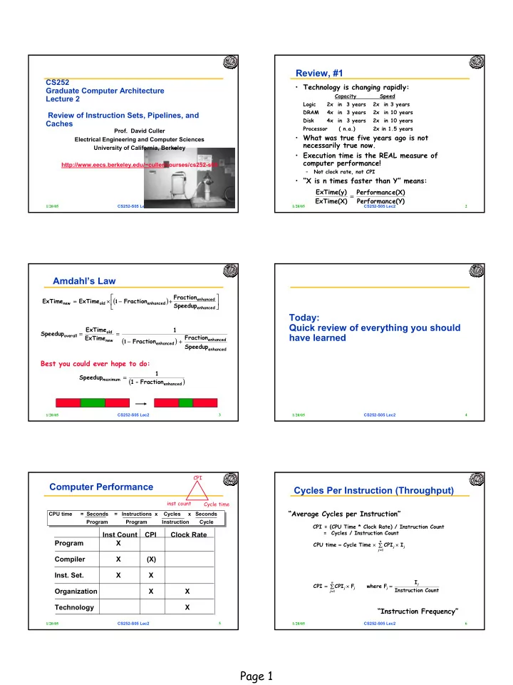
 Amdahl’s Law Fraction   ( ) ExTime ExTime Fraction enhanced = × − + 1   new old enhanced Speedup   enhanced Today: Quick review of everything you should ExTime 1 old Speedup = = overall have learned ExTime Fraction ( ) enhanced new − Fraction + 1 enhanced Speedup enhanced Best you could ever hope to do: 1 Speedup = maximum ( ) 1 - Fraction enhanced 1/20/05 CS252-S05 Lec2 3 1/20/05 CS252-S05 Lec2 4 CPI Computer Performance Cycles Per Instruction (Throughput) inst count Cycle time “Average Cycles per Instruction” CPU time = Seconds = Instructions x Cycles x Seconds CPU time = Seconds = Instructions x Cycles x Seconds Program Program Instruction Cycle Program Program Instruction Cycle CPI = (CPU Time * Clock Rate) / Instruction Count = Cycles / Instruction Count Inst Count CPI Clock Rate Program X n CPU time = Cycle Time × CPI × I ∑ j j j = 1 Compiler X (X) Inst. Set. X X I n CPI CPI F where F j = ∑ × = j j j Instructio n Count Organization X X = 1 j Technology X “Instruction Frequency” CS252-S05 Lec2 5 CS252-S05 Lec2 6 1/20/05 1/20/05 Page 1

  2. Example: Branch Stall Impact Example: Calculating CPI bottom up Run benchmark and collect workload characterization (simulate, machine • Assume CPI = 1.0 ignoring branches (ideal) counters, or sampling) • Assume solution was stalling for 3 cycles Base Machine (Reg / Reg) Op Freq Cycles CPI(i) (% Time) • If 30% branch, Stall 3 cycles on 30% ALU 50% 1 .5 (33%) Load 20% 2 .4 (27%) Op Freq Cycles CPI(i) (% Time) Store 10% 2 .2 (13%) Other 70% 1 .7 (37%) Branch 30% 4 1.2 (63%) Branch 20% 2 .4 (27%) ⇒ new CPI = 1.9 1.5 Typical Mix of instruction types in program • New machine is 1/1.9 = 0.52 times faster (i.e. slow!) Design guideline: Make the common case fast MIPS 1% rule: only consider adding an instruction of it is shown to add 1% performance improvement on reasonable benchmarks. 1/20/05 CS252-S05 Lec2 7 1/20/05 CS252-S05 Lec2 8 SPEC: System Performance Evaluation Cooperative SPEC First Round • One program: 99% of time in single line of code • First Round 1989 – 10 programs yielding a single number (“SPECmarks”) • New front-end compiler could improve dramatically • Second Round 1992 – SPECInt92 (6 integer programs) and SPECfp92 (14 floating point programs) » Compiler Flags unlimited. March 93 of DEC 4000 Model 610: spice: unix.c:/def=(sysv,has_bcopy,”bcopy(a,b,c)= 800 memcpy(b,a,c)” 700 wave5: /ali=(all,dcom=nat)/ag=a/ur=4/ur=200 600 nasa7: /norecu/ag=a/ur=4/ur2=200/lc=blas 500 • Third Round 1995 400 – new set of programs: SPECint95 (8 integer programs) and SPECfp95 (10 300 floating point) 200 – “benchmarks useful for 3 years” – Single flag setting for all programs: SPECint_base95, SPECfp_base95 100 • Fourth Round 2000: 26 apps 0 gcc doduc epresso spice nasa7 eqntott li fpppp tomcatv – analysis and simulation programs matrix300 – Compression: bzip2, gzip, – Integrated circuit layout, ray tracing, lots of others Benchmark 1/20/05 CS252-S05 Lec2 9 1/20/05 CS252-S05 Lec2 10 Integrated Circuits Costs A "Typical" RISC Die cost Testing cost Packaging cost + + IC cost = Final test yield • 32-bit fixed format instruction (3 formats) Wafer cost • 32 32-bit GPR (R0 contains zero, DP take pair) Die cost = Dies per Wafer × Die yield • 3-address, reg-reg arithmetic instruction 2 π (Wafer_dia m/2) π × Wafer_diam • Single address mode for load/store: Dies per wafer Test_Die = − − Die_Area 2 Die_Area ⋅ base + displacement – no indirection • Simple branch conditions • Delayed branch see: SPARC, MIPS, HP PA-Risc, DEC Alpha, IBM PowerPC, − α  Defect_Den sity Die_area    ×   CDC 6600, CDC 7600, Cray-1, Cray-2, Cray-3 Die Yield = Wafer_yiel d × 1 +       α     Die Cost goes roughly with die area 4 CS252-S05 Lec2 11 CS252-S05 Lec2 12 1/20/05 1/20/05 Page 2

  3. Example: MIPS (- DLX) Datapath vs Control Register-Register Datapath Controller 11 10 6 5 31 26 25 21 20 16 15 0 Op Rs1 Rs2 Rd Opx signals Register-Immediate 31 26 25 21 20 16 15 0 immediate Op Rs1 Rd Branch 31 26 25 21 20 16 15 0 immediate Op Rs1 Rs2/Opx Control Points Jump / Call • Datapath: Storage, FU, interconnect sufficient to perform the 31 26 25 0 desired functions target Op – Inputs are Control Points – Outputs are signals • Controller: State machine to orchestrate operation on the data path – Based on desired function and signals 1/20/05 CS252-S05 Lec2 13 1/20/05 CS252-S05 Lec2 14 5 Steps of DLX Datapath Approaching an ISA Figure 3.1, Page 130 • Instruction Set Architecture Instruction Instr. Decode Execute Memory Write – Defines set of operations, instruction format, hardware supported Fetch Reg. Fetch Addr. Calc Access Back data types, named storage, addressing modes, sequencing Next PC • Meaning of each instruction is described by RTL on MUX architected registers and memory Adder Next SEQ PC • Given technology constraints assemble adequate datapath 4 Zero? RS1 – Architected storage mapped to actual storage MUX MUX Address RS2 – Function units to do all the required operations Memory Reg File Inst – Possible additional storage (eg. MAR, MBR, …) ALU Memory L RD – Interconnect to move information among regs and FUs Data M MUX • Map each instruction to sequence of RTLs D • Collate sequences into symbolic controller state transition Sign diagram (STD) IR <= mem[PC]; Imm Extend • Lower symbolic STD to control points PC <= PC + 4 WB Data • Implement controller Reg[IR rd ] <= Reg[IR rs ] op IRop Reg[IR rt ] 1/20/05 CS252-S05 Lec2 15 1/20/05 CS252-S05 Lec2 16 5 Steps of DLX Datapath Inst. Set Processor Controller Figure 3.4, Page 134 Instruction Instr. Decode Execute Memory Write Fetch Reg. Fetch Addr. Calc Access Back IR <= mem[PC]; Ifetch Next PC PC <= PC + 4 MUX Next SEQ PC Next SEQ PC Adder 4 Zero? A <= Reg[IR rs ]; opFetch-DCD JSR RS1 JR ST B <= Reg[IR rt ] Address MUX MUX MEM/WB Memory RS2 Reg File EX/MEM jmp ID/EX IF/ID br LD RI ALU RR Memory r <= A + IR im Data r <= A op IRop IR im if bop(A,b) PC <= IR jaddr r <= A op IRop B MUX PC <= PC+IR im IR <= mem[PC]; WB Data Sign WB <= r WB <= r WB <= Mem[r] Extend Imm PC <= PC + 4 A <= Reg[IR rs ]; RD RD RD Reg[IR rd ] <= WB Reg[IR rd ] <= WB Reg[IR rd ] <= WB B <= Reg[IR rt ] rslt <= A op IRop B WB <= rslt CS252-S05 Lec2 17 CS252-S05 Lec2 18 1/20/05 1/20/05 Reg[IR rd ] <= WB Page 3

Download Presentation
Download Policy: The content available on the website is offered to you 'AS IS' for your personal information and use only. It cannot be commercialized, licensed, or distributed on other websites without prior consent from the author. To download a presentation, simply click this link. If you encounter any difficulties during the download process, it's possible that the publisher has removed the file from their server.

Recommend


More recommend