P ROBLEMS WITH I NCOMPLETE N ETWORKS : B IASES , S KEWED R ESULTS , - - PowerPoint PPT Presentation

p roblems with i ncomplete n etworks
SMART_READER_LITE
LIVE PREVIEW

P ROBLEMS WITH I NCOMPLETE N ETWORKS : B IASES , S KEWED R ESULTS , - - PowerPoint PPT Presentation

5/7/16 2016 SIAM SDM Tutorial 1 P ROBLEMS WITH I NCOMPLETE N ETWORKS : B IASES , S KEWED R ESULTS , AND S OLUTIONS Sucheta Tina Brian Ali Soundarajan Eliassi-Rad Gallagher Pinar Syracuse Northeastern Lawrence Sandia Natl University


slide-1
SLIDE 1

PROBLEMS WITH INCOMPLETE NETWORKS: BIASES, SKEWED RESULTS, AND SOLUTIONS

5/7/16 2016 SIAM SDM Tutorial 1

Sucheta Soundarajan Tina Eliassi-Rad Brian Gallagher Ali Pinar

Syracuse University Northeastern University Lawrence Livermore Nat’l Lab Sandia Nat’l Laboratories susounda@syr.edu tina@eliassi.org bgallagher@llnl.gov apinar@sandia.gov

slide-2
SLIDE 2

Complex networks are ubiquitous

Technological Networks Information Networks Social Networks Biological networks

Internet NY State Power Grid Map of Science Friendship HP Emails Contagion of TB Food Web

2

slide-3
SLIDE 3

Applications of complex networks

  • Link analysis and web search
  • Community detection
  • Classification on networks
  • Information maximization
  • Social recommendation
  • Epidemics
  • Cascades
  • ...

3

slide-4
SLIDE 4

Properties of complex networks

  • Size
  • Density
  • Average degree
  • Degree distribution
  • Average path length
  • Diameter of a network
  • Clustering coefficient
  • Connectedness
  • Node centrality

4

High School Dating (Bearman, Moody, and Stovel, 2004) (Image by Mark Newman)

slide-5
SLIDE 5

Properties of complex networks

  • Size
  • Density
  • Average degree
  • Degree distribution
  • Average path length
  • Diameter of a network
  • Clustering coefficient
  • Connectedness
  • Node centrality

5

slide-6
SLIDE 6

Properties of complex networks

  • Size
  • Density
  • Average degree
  • Degree distribution
  • Average path length
  • Diameter of a network
  • Clustering coefficient
  • Connectedness
  • Node centrality

6

slide-7
SLIDE 7

Properties of complex networks

  • Size
  • Density
  • Average degree
  • Degree distribution
  • Average path length
  • Diameter of a network
  • Clustering coefficient
  • Connectedness
  • Node centrality

7

slide-8
SLIDE 8

Properties of complex networks

  • Size
  • Density
  • Average degree
  • Degree distribution
  • Average path length
  • Diameter of a network
  • Clustering coefficient
  • Connectedness
  • Node centrality

8

http://arxiv.org/pdf/1111.4503.pdf

slide-9
SLIDE 9

Properties of complex networks

  • Size
  • Density
  • Average degree
  • Degree distribution
  • Average path length
  • Diameter of a network
  • Clustering coefficient
  • Connectedness
  • Node centrality
  • Node Influence

9

log-log scale

slide-10
SLIDE 10

Incomplete networks

  • Networked representations of

real-world phenomena are

  • ften partially observed
  • Acquiring more network data

is often expensive and/or hard

  • Even when your data is

complete, you may not have the computational resources to examine all of the data

10

slide-11
SLIDE 11

Roadmap

  • Introduction -- Tina
  • Part 1 -- Tina
  • Biases & Skewed Results
  • Part 2 -- Sucheta
  • Enhancing incomplete Networks
  • MaxOutProbe
  • MaxReach
  • ε-WGX
  • Wrap-up + Q&A -- Tina

11

slide-12
SLIDE 12

PART 1: BIASES & SKEWED RESULTS

12

slide-13
SLIDE 13

Partial observability

  • Data comes in increments
  • Tweets
  • Wall posts
  • Packets
  • Data is expensive or difficult to collect
  • Protein-protein interactions determined experimentally
  • Can’t place a monitor every where on the Internet

13

slide-14
SLIDE 14

Partial observability (cont.)

  • Data comes in increments
  • Data is expensive or

difficult to collect

  • Data is too big

14

slide-15
SLIDE 15

Resort to sampling

  • SDM 2015 Tutorial on Methods and Applications of Network

Sampling

  • Tutors: Mohammad A. Hasan, Nesreen K. Ahmed, and Jennifer

Neville

  • http://www.siam.org/meetings/sdm15/sampling.php

15

slide-16
SLIDE 16

Sampling

Access Scenarios

  • Complete access
  • Crawling access
  • Streaming access

Objectives

  • Sample to estimate

properties of the original network at the micro-, meso-, and/or macro-levels

  • Sample to obtain a small

(preferably unbiased) portion of the original network

16

slide-17
SLIDE 17

Sampling bias

  • Which nodes are most likely to be present in the sample?
  • High degree nodes
  • Low degree nodes

17

slide-18
SLIDE 18

Questions

  • How can we accurately estimate
  • the degree distribution
  • the average degree
  • the global clustering coefficient
  • f the underlying network using the sample?

18

slide-19
SLIDE 19

Commonly used sampling strategies

Random

  • Uniform random node

sampling (RNS)

  • Uniform random edge

sampling (RES)

Crawl

  • Random walk sampling

(RWS)

  • Breadth-first / snowball

sampling (BFS)

19

slide-20
SLIDE 20

Uniform random node sampling

1.

Select p fraction of nodes uniformly at random

2.

Include all edges adjacent to the selected nodes

  • Requires access to full list of nodes
  • All nodes are equally likely to be selected
  • High degree nodes are more likely to be observed as

neighbors of selected nodes

20

slide-21
SLIDE 21

Estimating degree distribution from a RNS

  • Provides unbiased estimates for any nodal property
  • Average degree
  • Average of any attribute on the nodes
  • Degree distribution
  • Disclaimer
  • If the sample is not the induced subgraph on the

randomly selected nodes, then it is unlikely to capture the distribution’s tail well

21

slide-22
SLIDE 22

Estimating clust. coeff. from a RNS

  • Use the sample to estimate
  • T = # of triangles in underlying network
  • W = # of wedges in underlying network
  • Clustering coefficient C = T / W

22

slide-23
SLIDE 23

Estimating number of triangles from a RNS

  • Probability that all three nodes are selected = p3
  • Probability that two of the three nodes are selected =

3p2(1 – p)

  • T =

23

Need at least two of these

Ts 3p2(1 – p) + p3

slide-24
SLIDE 24

Estimating the number of wedges from a RNS

  • Probability that center node is selected = p
  • Probability that endpoints, and not the center node, are

selected = p2(1 – p)

  • W =

24

W s p2(1 – p) + p

…or this Need at least two of these

slide-25
SLIDE 25

Estimating clust. coeff. from a RNS

Putting it all together… Ĉ = which is an unbiased estimator for C

25

(p(1 – p) + 1) 3p(1 – p) + p2 Ts W s ✕

slide-26
SLIDE 26

Uniform random edge sampling

  • 1. Select p fraction of edges uniformly at random

from the network

  • Requires access to full list of edges
  • All edges are equally likely to be selected
  • High degree nodes are more likely to be observed

26

slide-27
SLIDE 27

Estimating degree distribution from a RES

  • Degree distribution (and other statistics on nodes) will be

biased towards high-degree nodes

  • Edges statistics (such as assortativity) will be unbiased
  • Suppose a node u has degree du in the original network
  • Its degree in the sample is given by a binomial distribution

Bin(du, p)

  • Recall p is the fraction of edges chosen uniformly at

random

27

slide-28
SLIDE 28

Estimating degree distribution from a RES (cont.)

Solve a least squares problem, where matrix coefficients come from binomial distribution

28

Observed degree counts Estimated true degree counts A(i, j) = probability of node with true degree j having sample degree i

slide-29
SLIDE 29

Estimating clust. coeff. from a RES

  • Use the sample to estimate
  • T = # of triangles in underlying network
  • W = # of wedges in underlying network
  • Clustering coefficient C = T / W

29

slide-30
SLIDE 30

Estimating number of triangles from a RES

  • Probability that all three edges are selected = p3
  • T =

30

Need all three edges

Ts p

slide-31
SLIDE 31

Estimating number of wedges from a RES

  • Probability that both edges are selected = p2
  • W =

31

Need both edges

W s p2

slide-32
SLIDE 32

Estimating clust. coeff. from a RES

Putting it all together… Ĉ = which is an unbiased estimator for C

32

1 p Ts W s

slide-33
SLIDE 33

Random walk sampling

1.

Begin with a random start node

2.

At each step transition to a random neighbor of the current node

  • Do not need access to full set of nodes or edges ahead of

time (crawling)

  • In RW’s stationary distribution, probability of observing a

node u is proportional to du

  • P(u) = du / 2 |E|
  • High degree nodes are more likely to be present in the

sample

33

slide-34
SLIDE 34

Estimating structural properties from a RWS

If the random walk is long enough to be approximated by its stationary distribution then degree distribution and clustering coefficient can be estimated using the same procedure as random edge sample

34

slide-35
SLIDE 35

Breadth-first / snowball sampling

1.

Begin with a random start node (or random start nodes)

2.

Crawl the graph in a breadth-first fashion

  • Do not need access to full set of nodes/edges ahead of

time

  • Vanilla BFS provides a complete “snapshot” of one area
  • High degree nodes are more likely to be present in the

sample

  • Hard to estimate properties of underlying network from

sample

35

slide-36
SLIDE 36

Correcting biases in samples

  • Exploration based sampling is biased toward high degree

nodes

  • Can we modify the algorithms to ensure nodes are

sampled uniformly at random?

  • Yes, uniform node sampling with Metropolis-Hastings

method [Henzinger 2000]

  • Sampling algorithms that selects nodes non-uniformly are

biased when its comes to nodal statistics

  • Can we remove the sampling bias in nodal statistics by

post-processing?

  • Yes, see Salganik & Heckathorn 2004

36

From Hasan, Ahmed, and Neville, SDM’15 Tutorial.

slide-37
SLIDE 37

Roadmap

  • Introduction -- Tina
  • Part 1 -- Tina
  • Biases & Skewed Results
  • Part 2 -- Sucheta
  • Enhancing incomplete Networks
  • MaxOutProbe
  • MaxReach
  • ε-WGX
  • Wrap-up + Q&A -- Tina

37

slide-38
SLIDE 38

PART 2: ENHANCING INCOMPLETE NETWORKS

38

slide-39
SLIDE 39

Research question

Given limited resources, how should one gather more data to get the most bang for the buck? Two approaches:

  • 1. Model aware
  • 2. Model agnostic

39

slide-40
SLIDE 40

Given limited resources, how should one gather more data to get the most bang for the buck?

Model Aware

  • Don’t gather more data
  • Assume a graph model
  • Use the incomplete network

to fit a model of network structure

  • Infer missing data
  • A.k.a. network completion

problem

40

slide-41
SLIDE 41

The network completion problem

Given part of an adjacency matrix, infer the rest of the matrix

41

  • M. Kim, J. Leskovec: The Network Completion Problem: Inferring Missing Nodes and Edges in Networks.

In SDM 2011: 47-58

From Kim & Leskovec, SDM 2011

slide-42
SLIDE 42

Examples of network completion

Hanneke & Xing [AISTATS’09]

  • Assume survey sample (nodes +

neighbors)

  • Assume stochastic block model
  • Assume that block memberships
  • f surveyed nodes are known
  • Use observed data to estimate

block connection probabilities

  • Gives probability that two

nodes are connected

Kim & Leskovec [SDM’11]

  • Assume Kronecker graph model
  • Cast problem in EM framework
  • Given observed data, use a

Metropolized Gibbs sampling method to estimate parameters

  • f model and infer missing data

42

  • Steve Hanneke, Eric P. Xing: Network Completion and Survey Sampling. In AISTATS 2009: 209-215
  • M. Kim, J. Leskovec: The Network Completion Problem: Inferring Missing Nodes and Edges in Networks.

In SDM 2011: 47-58

slide-43
SLIDE 43

The network inference problem

  • Related to network completion
  • Infer the network over which contagions propagate
  • Lots of recent activity in this area
  • Eldar Sadikov, Montserrat Medina, Jure Leskovec, Hector Garcia-Molina:

Correcting for missing data in information cascades. In WSDM 2011: 55-64

  • Manuel Gomez-Rodriguez, David Balduzzi, Bernhard Schölkopf:

Uncovering the Temporal Dynamics of Diffusion Networks. In ICML 2011: 561-568

  • Manuel Gomez-Rodriguez, Jure Leskovec, Andreas Krause:

Inferring Networks of Diffusion and Influence. TKDD 5(4): 21 (2012)

  • Nan Du, Le Song, Ming Yuan, Alex J. Smola: Learning Networks of

Heterogeneous Influence. In NIPS 25, 2012: 2789--2797

  • Bruno D. Abrahao, Flavio Chierichetti, Robert Kleinberg, Alessandro

Panconesi: Trace complexity of network inference. In KDD 2013: 491-499

43

slide-44
SLIDE 44

Given limited resources, how should one gather more data to get the most bang for the buck?

Model Aware

  • Don’t gather more data
  • Assume a graph model
  • Use the incomplete network

to fit a model of network structure

  • Infer missing data
  • A.k.a. network completion

problem

Model Agnostic

  • Don’t assume a model

44

slide-45
SLIDE 45

Model agnostic approaches may be worth considering when no model fits

45

degree 10^0

10^1 10^2 10^3

CCDF

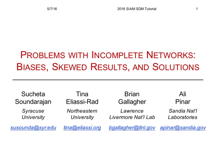
10^−3 10^−2 10^−1 10^0 ground truth DIMES IP iPlane IP iPlane R Ark AllPref IP Ark ITDK R mi Ark ITDK R mik

(c) The CCDF of node degrees for each processing method and data source.

* B. Huffaker, M. Fomenkov, and K.C. Claffy. Internet topology data comparison. CAIDA Report, 2012. http://www.caida.org/publications/papers/2012/topocompare-tr/topocompare-tr.pdf

Inferred degree distributions of various methods vs. ground truth (red).* None of the approaches provide confidences or guarantees on their results. Ongoing work with C. Seshadhri @ UCSC: Property testing in sparse graphs with realistic characteristics

slide-46
SLIDE 46

Given limited resources, how should one gather more data to get the most bang for the buck?

Model Aware

  • Don’t gather more data
  • Assume a graph model
  • Use the incomplete network

to fit a model of network structure

  • Infer missing data
  • A.k.a. network completion

problem

Model Agnostic

  • Don’t assume a model
  • Infer missing data (e.g., link

prediction) OR

  • Collect additional data

46

slide-47
SLIDE 47

Given limited resources, how should one gather more data to get the most bang for the buck?

Model Aware

  • Don’t gather more data
  • Assume a graph model
  • Use the incomplete network

to fit a model of network structure

  • Infer missing data
  • A.k.a. network completion

problem

Model Agnostic

  • Don’t assume a model
  • Infer missing data (e.g., link

prediction) OR

  • Collect additional data

47

Focus of this tutorial

slide-48
SLIDE 48

Issues to consider

Goal

  • Observe as many new nodes

as possible

  • Find triangles in the incomplete

network

  • Find links between “external”

nodes

  • ...

Access Models

  • Types of queries allowed
  • Can ask for:
  • all the edges of a node
  • a random edge of a node
  • k random edges of a nodes
  • all the communications

between two nodes

48

?

slide-49
SLIDE 49

Roadmap for Part 2

  • MaxOutProbe: A heuristic approach
  • Goal: Observe as many new nodes as possible
  • Query: Returns all the edges of a node
  • MaxReach: A heuristic approach
  • Goal: Observe as many new nodes as possible
  • Query: Returns all edges, k edges, or requested # edges
  • ε-WGX: A multi-armed bandit approach
  • Goal: Observe as many new nodes as possible
  • Query: Returns a random edges of a node

49

slide-50
SLIDE 50

50

slide-51
SLIDE 51

MaxOutProbe: Problem definition

  • Given
  • An incomplete network Ĝ that is part of a larger, unseen

network G

  • A probing budget b in
  • Goal
  • Select b nodes from Ĝ that, when probed, bring as many

new nodes as possible into Ĝ

  • Assumption
  • When a node is probed, all of its neighbors from G are
  • bserved

51

slide-52
SLIDE 52

Running example: Ĝ

52

slide-53
SLIDE 53

Running example

53

In Ĝ In G, but not in Ĝ

Which yellow nodes are adjacent to many green nodes?

slide-54
SLIDE 54

Running example: Which yellow nodes are adjacent to many green nodes?

54

In Ĝ In G, but not in Ĝ

slide-55
SLIDE 55

MaxOutProbe: Outline

  • 1. Using Ĝ, estimate each node u’s true degree du

in G

  • 2. Estimate the number of neighbors u has inside Ĝ
  • Using Ĝ, estimate the average clustering

coefficient C of G

  • 3. Using #1 and #2, estimate the number of

neighbors u has outside Ĝ

55

slide-56
SLIDE 56

MaxOutProbe (cont.)

56

du

  • ut = du −du

in = du − du known +du unknown

( )

u

In Ĝ In G, but not in Ĝ

slide-57
SLIDE 57

Estimating degree of a node du

  • Hypothesis
  • There is a scaling factor s such that a node’s

true degree can be approximated by s times its observed degree

  • How do we calculate s?
  • Sample a small number of high degree nodes

from Ĝ

  • Observe the ratio of their true degrees to their
  • bserved degrees

57

slide-58
SLIDE 58

Estimating internal degrees

  • Challenge
  • Given the structure of Ĝ, how can we estimate

the number of neighbors a node has inside Ĝ?

  • Observation: Nodes tend to cluster
  • If u has many friends-of-friends inside Ĝ,

chances are u is connected to some of them

  • How many?
  • Use clustering coefficient to figure it out
  • Among the wedges, what fraction are closed

triangles?

58

slide-59
SLIDE 59

Running example

  • u has 4 friends-of-friends (red-lined yellow circles)
  • C = estimate of graph’s clustering coefficient
  • Estimate that u is connected to

4C of these nodes

59

u

? ? ? ?

u

slide-60
SLIDE 60

Estimating C

  • Reuse nodes probed during degree-estimation

step

  • When probed, what fraction of their friends-of-

friends were they connected to?

60

slide-61
SLIDE 61

Unbiased estimates

  • MaxOutProbe obtains unbiased estimates if we know that
  • Ĝ was produced by sampling nodes or edges uniformly at

random from G and

  • the size of G
  • Details at http://arxiv.org/pdf/1511.06463v1.pdf

61

slide-62
SLIDE 62

62

slide-63
SLIDE 63

Datasets

63

Network # of Nodes # of Edges

Transitivity

Twitter Retweets 40K 46K 0.03 Twitter Replies 261K 309K 0.002 Enron Emails 84K 326K 0.08 Yahoo! IM 100K 595K 0.08 Amazon Books 270K 741K 0.21 Youtube Videos 167K 1M 0.007

slide-64
SLIDE 64

Baseline & competing methods

64

Name Description HighDeg LowDeg HighDisp LowDisp CrossCom HighCC LowCC Select nodes with the highest degree. Select nodes with the lowest degree. Select nodes with the highest dispersion. Select nodes with the lowest dispersion. Select nodes with the highest fraction of neighbors outside

  • f their community (detected by Louvain Method).

Select nodes with the highest clustering coefficients. Select nodes with the lowest clustering coefficients. Random Randomly select nodes from the sample.

slide-65
SLIDE 65

Experimental setup

  • 20 trials
  • Sample 10% of G’s edges using:
  • Random node sampling
  • Random edge sampling
  • Random walk
  • Random walk with jumps
  • Run experiments at budgets b

in {1%, 2%, 3%, 4%, 5%} of the # of nodes in each network

  • Evaluate the quality of the enhanced graph by counting how

many nodes it has

65

slide-66
SLIDE 66

MaxOutProbe: Results

1.

Compared to random probing, MaxOutProbe outperforms High Degree probing (the best baseline) by 4% - 36% on average

2.

Small improvements are because of tiny clustering coefficients

66

Twitter Replies, C = 0.002, Random Walk

Enron e-mail, C = 0.08, Random Edge

slide-67
SLIDE 67

MaxOutProbe: Summary

  • Goal: Observe as many new nodes as possible
  • Query: Returns all the edges of a node
  • MaxOutProbe
  • Makes no assumptions about how the incomplete graph with

generated or observed

  • Takes clustering coefficient into account
  • Improves performance over the best baseline algorithm

(i.e., high-degree) by 4% to 36%

  • Improvement depends on G’s clustering coefficient
  • Tiny C, less improvement

67

Sucheta Soundarajan, Tina Eliassi-Rad, Brian Gallagher, Ali Pinar: MaxOutProbe: An Algorithm for Increasing the Size of Partially Observed Networks. 2015 NIPS Workshop on Networks in the Social and Information Sciences. http://arxiv.org/abs/1511.06463

slide-68
SLIDE 68

68

slide-69
SLIDE 69

MaxReach

  • Similar problem definition as in MaxOutProbe
  • Given
  • An incomplete network Ĝ that is part of a larger, unseen

network G

  • A probing budget b in
  • Goal
  • Select b nodes from the evolving Ĝ that, when probed,

bring as many new nodes as possible into the current Ĝ

69

slide-70
SLIDE 70

MaxReach improves MaxOutProbe

  • 1. Allows probing of new nodes as they are
  • bserved
  • 2. Flexible access model
  • Example: Does not require all the edges of a probed

node to be returned

  • 3. More accurate degree and clustering coefficient

estimates

70

slide-71
SLIDE 71

MaxReach assumptions

  • Ĝ was produced by random node or random edge

sample; and we know which

  • We know the size of G
  • # of nodes and # of edges

71

slide-72
SLIDE 72

MaxReach improves degree estimates

  • Suppose Ĝ was produced by sampling p fraction of edges

from G

  • To estimate the degree distribution of G, solve the following

least squares problem

72

B(i, j) = Prob. that node with degree j in G has degree i in Ĝ Degree counts in G (to be estimated) Degree counts in Ĝ

slide-73
SLIDE 73

MaxReach improves degree estimates

  • Our least squares problem is underdetermined
  • Instead, use an EM-like iterative process to estimate the

degree counts in G

73

Initialize to uniform degree distribution Estimate each node’s true degree Update degree distribution

Iterative Estimation Process

slide-74
SLIDE 74

MaxReachimproves degree estimates

  • Calculate K-L divergence of the estimated degree

distribution vs. the true distribution

  • MaxReach performs 24-430✕ better than

MaxOutProbe

74

slide-75
SLIDE 75

MaxReachimproves clust. coeff. estimates

  • Clustering coefficient is related to degree

75

slide-76
SLIDE 76

MaxReachimproves clust. coeff. estimates

  • Probability a wedge is preserved in Ĝ = p2
  • Probability a triangle is preserved in Ĝ = p3
  • Estimated CC = (Observed CC)/p

76

u

Preserved triangle Preserved wedge but lost triangle Lost wedge & triangle

slide-77
SLIDE 77

MaxReach improves clust. coeff. estimates

  • MaxOutProbe estimates the global average clust. coeff.
  • MaxReach estimates a per-degree average clust. coeff.

77

slide-78
SLIDE 78

MaxReach estimates node statistics

1.

Estimate each node u’s true degree in G (i.e., du) by using

  • estimated degree distribution, and
  • u’s observed degree in Ĝ

2.

Estimate the number of neighbors u has inside Ĝ (i.e., duin) by using

  • estimated clustering coefficients of observed neighbors

in Ĝ

3.

Estimate the number of neighbors u has outside Ĝ (i.e., duout) by using the estimates in #1 and #2

78

slide-79
SLIDE 79

What is the access model?

  • 1. All of a node’s edges?
  • Example: Facebook Graph API
  • 2. k of a node’s edges?
  • Example: Twitter API returns 5000 neighbors
  • 3. A requested number of edges?
  • Assumption: There is a cost to initiate the request

79

slide-80
SLIDE 80

MaxReach scores each node

  • All of a node’s edges?
  • Score(u) = duout
  • k of a node’s edges?
  • Score(u) = min{k, du – duknown} ✕ (duout ⁄ (du – duknown))
  • A requested number of edges, with a cost to initiate the

request?

  • Score(u) = maxk ( (k duout) ⁄ ((du – duknown) (rk + c)) )
  • k = # of requested edges, such that k ≤ du – duknown
  • c = request charge
  • r = cost per edges

80

slide-81
SLIDE 81

MaxReach’s update step

  • MaxReach updates node scores incrementally
  • Allows us to make estimates for nodes as they are

added to Ĝ

  • What is the expected degree of node u given
  • its original observed degree in Ĝ, and
  • the fact that its true degree ≥ its observed degree?
  • Solution: Use Bayes’ Theorem and prior probabilities from

G’s estimated degree distribution

81

slide-82
SLIDE 82

82

slide-83
SLIDE 83

Datasets

83

Network # of Nodes # of Edges

Transitivity

Twitter Retweets 40K 46K 0.03 Twitter Replies 261K 309K 0.002 Enron Emails 84K 326K 0.08 Yahoo! IM 100K 595K 0.08 Amazon Books 270K 741K 0.21 DBLP 317K 1M 0.31

slide-84
SLIDE 84

Experimental setup

  • 10 trials
  • Sample 10% of G’s edges using
  • Random node sampling
  • Random edge sampling
  • Run experiments at various budgets
  • Budget depends on access model
  • Evaluate quality of the enhanced graph by counting how

many nodes it has

  • Compare with adaptive versions of High Degree, Low

Degree, and Random Probing

84

slide-85
SLIDE 85

MaxReach: Results

On average, over all access models, MaxReach

  • utperforms all baseline strategies

85

All-neighbor Probing 5-random-neighbor Probing

slide-86
SLIDE 86

MaxReach: Summary of Results

86

All-neighbor access model k-neighbor access model Connection charge access model MaxReach

  • utperforms

Adaptive High Degree Probing by 57-61% 9-59% 28-46%

slide-87
SLIDE 87
  • Goal: Bring in as many nodes as possible
  • MaxReach
  • Works under a variety of access models
  • Requires that the incomplete network was
  • bserved via random node or random edge

sampling

  • Consistently outperforms other approaches

when the goal is to increase # of nodes

87

MaxReach: Summary

  • S. Soundarajan, T. Eliassi-Rad, B. Gallagher, A. Pinar: MaxReach: Reducing Network Incompleteness

through Node Probes, Technical Report, April 2016 (currently under peer-review)

slide-88
SLIDE 88

88

slide-89
SLIDE 89

ε-WGX: Problem definition

  • Adaptive Edge Probing (AEP)
  • Given
  • Incomplete network Ĝ that is part of a larger, unseen

network G

  • Probing budget b in
  • Reward function R : (u, v) → (ru, r’

v), where ru , r’ v in

  • Goal
  • Incrementally select b nodes in Ĝ that, when probed,

produce a graph Ĝ’, where Ĝ in Ĝ’ and Ĝ’ maximizes cumulative reward

  • Assumption
  • When a node is probed, one of its edges in G is selected

uniformly at random, including edges seen before

89

slide-90
SLIDE 90

Challenges and questions for AEP

  • No prior knowledge of how Ĝ was observed or generated
  • Using only a node’s observed links in Ĝ
  • When to stop probing a node?
  • Is there a general approach that works well across different

reward functions and graphs from various domains?

90

slide-91
SLIDE 91

Multi-armed bandits

91

A multi-armed bandit is a tuple hA, Ri A is a known set of m actions (or “arms”) Ra(r) = P [r|a] is an unknown probability distribution over rewards At each step t the agent selects an action at 2 A The environment generates a reward rt ⇠ Rat The goal is to maximise cumulative reward Pt

τ=1 rτ

Slide Courtesy of David Silver, UCL

slide-92
SLIDE 92

Exploration vs. exploitation

Exploration

  • Pick an arm at

random

  • So, gather more

information

Exploitation

  • Pick the arm that

maximizes reward given current information

  • So, make the best

decision

92

slide-93
SLIDE 93

MAB is a promising approach for AEP

  • Can be used without background knowledge of

network structure

  • Can adapt to different reward function
  • Is regularly providing the best performance for any

given network and reward function

  • Disclaimer: based on our preliminary results

93

slide-94
SLIDE 94

Some previous work on MAB with feedback graphs / side observations

  • Leveraging Side Observations in Stochastic Bandits by

Stéphane Caron, et al. 2012

  • Nonstochastic Multi-Armed Bandits with Graph-Structured

Feedback by Noga Alon, et al. 2014

  • Online Learning with Feedback Graphs: Beyond Bandits by

Noga Alon et al. 2015

94

slide-95
SLIDE 95

Challenges in using MAB for AEP

  • Changing rewards
  • Probability of getting a new edge decreases as a node is

probed more

  • The graph itself can be changing
  • Complementarities: rewards depend on each other, even

if those two nodes are not directly connected

  • Short lifespan on bandits
  • Number of useful probes on any one node is likely to be

small

  • New arms get added

95

slide-96
SLIDE 96

Graph complementarities

  • Initially, r*(u) = ½ and r*(v) = ½
  • I.e., both u and v have half of

their neighbors outside Ĝ

  • If we probe node u and get

edge (u, w), r*(u) = 0 and r*(v) = 0

  • There is nothing left to learn

for u

  • Because we have already seen

node w, there is nothing left to learn for v as well

96

u v w y Ĝ

r* = true reward

slide-97
SLIDE 97

ε-WGX: A nested bandit algorithm

97

Outer Bandit Inner Bandit Explore unprobed nodes Explore Exploit Exploit Explore all nodes ε1 1−ε1 0.5 0.5 ε0 1−ε0

slide-98
SLIDE 98

Important aspects of ε-WGX

  • 1. Different rewards for a node
  • One reward for when it is probed directly
  • Another reward for when it is observed as a

neighbor

  • 2. Probability of seeing a new edge from a node

probe

99

slide-99
SLIDE 99

Once a probe is made…

  • ε-WGX updates

1.

ru = empirical mean reward for u which includes when u was probed and when it was

  • bserved as a neighbor

2.

pu = probability of seeing a new edge if u is probed again

3.

rv, if the observed neighbor v was already in the

  • bserved network
  • Expected reward of a node u = pu × ru

100

slide-100
SLIDE 100

Calculating pu

  • pu = probability of seeing a new edge when u is probed
  • Suppose node u has been probed k times with w distinct

neighbors and h duplicates è k = w + h

  • What is the estimated degree d of node u?
  • Same as predicting population size with random draws [Samuel

1968]

  • MLE of d is:
  • Assuming all edges are equally likely to be observed by a probe

101

* E. Samuel. Sequential maximum likelihood estimation of the size of a population. Annals of Mathematical Statistics, 39(3):1057–1068, 1968.

d

! = w+h

m

w k

( )

, where m(s) is the solution to w k = 1−e−m m

pu =1−w d

!

Details

slide-101
SLIDE 101

ε-WGX: Algorithmic Overview

102

  • For each node u, keep track of the time-step that it was first observed, T(u);

each node u in Ĝ has a T(u) = 0

  • While within budget b
  • Select a node u for probing according to the nested bandit probabilities
  • Node u is probed and edge (u, v) is obtained
  • If v is a newly observed node
  • Set T(v) = current time step
  • Add 1 to the cumulative sum for ru and increment its running count
  • Otherwise

/* v was observed previously */

  • If T(v) > T(u)

/* v was observed after u */

  • Add 1 to the cumulative sum for ru
  • Add 0 to the cumulative sum for r’v
  • Otherwise

/* v was observed before u */

  • Add 0 to the cumulative sum for ru
  • Add 1 to the cumulative sum for r’v
  • Increment the running counts for u and v
  • Update ru , rv(if necessary), pu

Details

slide-102
SLIDE 102

ε-WGX’s Regret

103

  • Regret after T time steps = expectation of the cumulative

difference the estimated reward and the optimal reward

  • The optimal policy knows which arms are best to play

and how the arms affect each others rewards

  • ε-WGX has linear regret (similar to ε-greedy)
  • ε-WGX explores a constant fraction of the time
  • ε-WGX assumes a static graph so the above does not

hold as time goes infinity

  • Why? As time goes to infinity, regret goes to zero

– i.e., you will get the complete graph

slide-103
SLIDE 103

104

slide-104
SLIDE 104

Datasets

105

Network G # of Nodes # of Edges G’s Avg.

  • Clust. Coeff.

FB Grad 0.5K 3.3K 0.48 FB Ugrad 1.2K 43K 0.30 Twitter Retweet 40K 46K 0.14 FB Social Circles 4K 88K 0.61 Twitter Replies 261K 309K 0.004 Enron Emails 84K 326K 0.15 Amazon Books 270K 741K 0.40

slide-105
SLIDE 105

Baseline & competing methods

  • ε-greedy
  • Upper Confidence Bound (UCB)
  • High degree
  • Low degree
  • Random

106

slide-106
SLIDE 106

Experimental setup: Incomplete graphs

  • Sample 10% of G’s edges using:
  • Breadth-first crawl
  • Random edge sampling
  • Random walk
  • Random walk with jumps

107

slide-107
SLIDE 107

Experimental setup: Probing budget

108

  • Ĝ = incomplete graph
  • G = complete graph
  • K = # of edges in G that are adjacent to at least one node

in Ĝ

  • M = K – # of edges in Ĝ
  • M = # of edges that include nodes from Ĝ, but have not

yet been observed.

  • Budget increments are the 100-quantiles in [cmin× M, cmax× M]

Details

slide-108
SLIDE 108

Experimental setup: Exploration parameters

  • Largely empirical
  • Similar to ε-greedy
  • Outer bandit has two choices: prioritize unprobed nodes or not
  • Its exploration parameter set to 0.05
  • This parameter could be implemented with decay
  • Inner bandit has many choices: which specific node to select
  • Its exploration parameter set to 0.3
  • This parameter should not decay

109

slide-109
SLIDE 109

Evaluation

  • 10 trials
  • For each network & probing budget b
  • Calculate how much ε-WGX increased the # of nodes,

divided by how much the comparative algorithm increased # of nodes

110

V

! 'εWGX −V !

V

! 'comp−V !

slide-110
SLIDE 110

ε-WGX: Results

  • Goal: Observe as many new nodes as possible
  • Query: Returns a random edges of a node

111

Incomplete network observed via BFS RandEdge RW RWJ Random 92% 76% 83% 80% Low Degree (Best Baseline) 91% 86% 93% 88% ε-Greedy 92% 86% 87% 73% UCB 80% 83% 87% 84% How Often Does ε-WGX Beat Other Methods?

slide-111
SLIDE 111
  • Adaptive Edge Probing (AEP) Problem
  • MAB for AEP
  • ε-WGX: nested MAB algorithm; model agnostic
  • Regularly outperforms other approaches when the

goal is to increase # of nodes

  • Lots more work to be done
  • Collective classification of reward/regret
  • Dynamic graphs

112

ε-WGX: Summary

  • S. Soundarajan, T. Eliassi-Rad, B. Gallagher, A. Pinar: Multi-armed Bandits for Enhancing Incomplete

Networks, Working Paper, May 2016

slide-112
SLIDE 112

Roadmap

  • Introduction -- Tina
  • Part 1 -- Tina
  • Biases & Skewed Results
  • Part 2 -- Sucheta
  • Enhancing incomplete Networks
  • MaxOutProbe
  • MaxReach
  • ε-WGX
  • Wrap-up + Q&A -- Tina

113

slide-113
SLIDE 113

Wrap-up

  • Beware your networked data is incomplete
  • Mining can lead to skewed results
  • Model-aware solution
  • Don’t gather data
  • Assume a model
  • Use the incomplete network

to fit a model of network structure

  • Model-agnostic solution
  • Estimate local and/or global network statistics
  • Gather data based on your estimates
  • Repeat until out of budget

114

Focus of this tutorial

slide-114
SLIDE 114

Future work

  • Model aware + data gathering
  • MAB for enhancing incomplete networks
  • Handling incomplete dynamic graphs
  • Treating the graph as a constrained network
  • Full observability in parts of the graph but partial in other

parts

  • Semantics of a non-edge

115

slide-115
SLIDE 115

Thank you

  • Slides and resources at

http://eliassi.org/sdm16tut.html

  • WIND’16: Workshop on

Incomplete Networked Data

  • http://eliassi.org/WIND16.html
  • Contact us at
  • susounda@syr.edu
  • tina@eliassi.org
  • Supported by NSF, DTRA,

DARPA, LLNL, and Sandia.

116