Overview Model Comparison Machine Learning and Pattern Recognition - - PowerPoint PPT Presentation

Model Comparison

Machine Learning and Pattern Recognition Chris Williams

School of Informatics, University of Edinburgh

October 2014

(These slides have been adapted from previous versions by Charles Sutton, Amos Storkey and David Barber

1 / 20

Overview

◮ The model selection problem ◮ Overfitting ◮ Validation set, cross validation ◮ Bayesian Model Comparison ◮ Reading: Murphy 1.4.7, 1.4.8, 6.5.3, 5.3; Barber 12.1-12.4,

13.2 up to end of 13.2.2

2 / 20

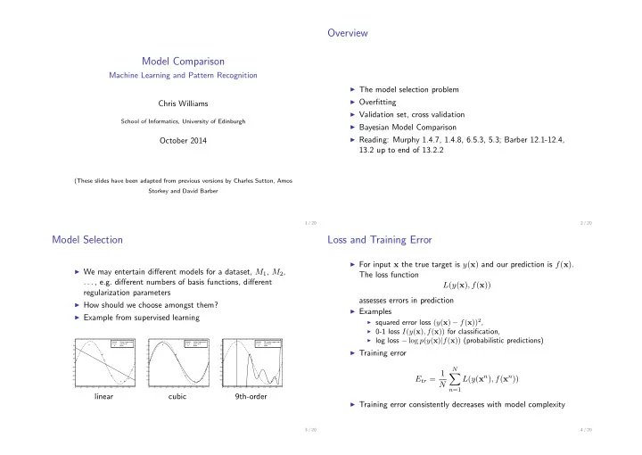
Model Selection

◮ We may entertain different models for a dataset, M1, M2,

. . . , e.g. different numbers of basis functions, different regularization parameters

◮ How should we choose amongst them? ◮ Example from supervised learning

0.1 0.2 0.3 0.4 0.5 0.6 0.7 0.8 0.9 1 −1 −0.8 −0.6 −0.4 −0.2 0.2 0.4 0.6 0.8 1

linear regression sin(2 π x) data

0.1 0.2 0.3 0.4 0.5 0.6 0.7 0.8 0.9 1 −1 −0.8 −0.6 −0.4 −0.2 0.2 0.4 0.6 0.8 1

cubic regression sin(2 π x) data

0.1 0.2 0.3 0.4 0.5 0.6 0.7 0.8 0.9 1 −1 −0.8 −0.6 −0.4 −0.2 0.2 0.4 0.6 0.8 1

9th−order regression sin(2 π x) data

linear cubic 9th-order

3 / 20

Loss and Training Error

◮ For input x the true target is y(x) and our prediction is f(x).

The loss function L(y(x), f(x)) assesses errors in prediction

◮ Examples

◮ squared error loss (y(x) − f(x))2, ◮ 0-1 loss I(y(x), f(x)) for classification, ◮ log loss − log p(y(x)|f(x)) (probabilistic predictions)

◮ Training error

Etr = 1 N

N

• n=1

L(y(xn), f(xn))

◮ Training error consistently decreases with model complexity

4 / 20

Overfitting

◮ Generalization (or test) error

Egen =

• L(y(x), f(x)) p(x, y) dx dy

◮ Overfitting (Mitchell 1997, p. 67)

A hypothesis f is said to overfit the data if there exists some alternative hypothesis f′ such that f has a smaller training error than f′, but f′ has a smaller generalization error than f.

5 / 20

Validation Set

◮ Partition the available data into two: a training set (for fitting

the model), and a validation set (aka hold-out set) for assessing performance

◮ Estimate the generalization error with

Eval = 1 V

V

• v=1

L(y(xv), f(xv)) where we sum over cases in the validation set

◮ Unbiased estimator of the generalization error ◮ Suggested split: 70% training, 30% validation

6 / 20

Cross Validation

◮ Split the data into K pieces (folds) ◮ Train on K − 1, test on the remaining fold ◮ Cycle through, using each fold for testing once ◮ Uses all data for testing, cf. the hold-out method

Figure credit: Murphy Fig 1.21(b) 7 / 20

Cross Validation: Example

5 10 15 20 −10 −5 5 10 15 20 ln lambda −20.135 5 10 15 20 −15 −10 −5 5 10 15 20 ln lambda −8.571

Figure credit: Murphy Fig 7.7

◮ Degree 14 polynomial with N = 21 datapoints ◮ Regularization term λwT w ◮ How to choose λ?

8 / 20

−25 −20 −15 −10 −5 5 5 10 15 20 25 log lambda mean squared error train mse test mse

−20 −15 −10 −5 5 0.1 0.2 0.3 0.4 0.5 0.6 0.7 0.8 0.9 log lambda negative log marg. likelihood CV estimate of MSE

Figure credit: Murphy Fig 7.7

◮ Left-hand end of x-axis ≡ low regularization ◮ Notice that training error increases monotonically with λ ◮ Miminum of test error is for an intermediate value of λ ◮ Both cross validation and a Bayesian procudure (coming

soon) choose regularized models

9 / 20

Bayesian Model Comparison

◮ Have a set of different possible models

Mi ≡ p(D|θ, Mi) and p(θ|Mi) for i = 1, . . . , K

◮ Each model is set of distributions that have associated

• parameters. Usually some models are more complex (have

more parameters) than others

◮ Bayesian way: Have a prior p(Mi) over the set of models Mi,

then compute posterior p(Mi|D) using Bayes’ rule p(Mi|D) = p(Mi)p(D|Mi) K

j=1 p(Mj)p(D|Mj) ◮

p(D|M) =

• p(D|θ, M)p(θ|M) dθ

This is called the marginal likelihood or the evidence.

10 / 20

Comparing models

Bayes factor = P(D|M1) P(D|M2) P(M1|D) P(M2|D) = P(M1) P(M2).P(D|M1) P(D|M2) Posterior ratio = Prior ratio × Bayes factor Strength of evidence from Bayes factor (Kass, 1995; after Jeffreys, 1961) 1 to 3 Not worth more than a bare mention 3 to 20 Positive 20 to 150 Strong > 150 Very strong

11 / 20

Computing the Marginal Likelihood

◮ Exact for conjugate exponential models, e.g. beta-binomial,

Dirichlet-multinomial, Gaussian-Gaussian (for fixed variances)

◮ E.g. for Dirichlet-multinomial

p(D|M) = Γ(α) Γ(α + N)

r

• i=1

Γ(αi + Ni) Γ(αi)

◮ Also exact for (generalized) linear regression (for fixed prior

and noise variances)

◮ Otherwise various approximations (analytic and Monte Carlo)

are possible

12 / 20

BIC approximation

BIC = log p(D|ˆ θ) − dof(ˆ θ) 2 log N

◮ Bayesian information criterion (Schwarz, 1978) ◮ ˆ

θ is MLE

◮ dof(ˆ

θ) is the degrees of freedom in the model (∼ number of parameters in the model)

◮ BIC penalizes ML score by a penalty term ◮ BIC is quite a crude approximation to the marginal likelihood

13 / 20

◮ Why Bayesian model selection? Why not compute best fit

parameters and compare?

◮ More parameters=better fit to data. ML: bigger is better. ◮ But might be overfitting: only these parameters work. Many

• thers don’t.

◮ Prefer models that are unlikely to ‘accidentally’ explain the

data.

14 / 20

Binomial Example

Example

You are an auditor of a firm. You receive details about the sales that a particular salesman is making. He attempts to make 4 sales a day to independent companies. You receive a list

• f the number of sales by this agent made on a number of days.

Explain why you would expect the total number of sales to be binomially distributed. If the agent was making the sales numbers up as part of a fraud, you might expect the agent (as he is a bit dim) to choose the number of sales at random from a uniform distribution. You are aware of the fraud possibility, and you understand there is something like a 1/5 chance this salesman is involved. Given daily sales counts of 1 2 2 4 1 4 3 2 4 1 3 3 2 4 3 3 2 3 3, do you think the salesman is lying?

15 / 20

Binomial Example

Example

Data: 1 2 2 4 1 4 3 2 4 1 3 3 2 4 3 3 2 3 3

◮ M = 1 - From P1(x|p) a binomial distribution Binomial(4).

Prior on p is uniform.

◮ M = 2 - From P2(x) a uniform distribution Uniform(0,. . . ,4). ◮ Discuss what you would do? ◮ P(M = 1) = 0.8.

16 / 20

Binomial Example

Example

Data: 1 2 2 4 1 4 3 2 4 1 3 3 2 4 3 3 2 3 3

◮ M = 1 - From P1(x|p) a binomial distribution Binomial(4).

Prior on p is uniform.

◮ M = 2 - From P2(x) a uniform distribution Uniform(0,. . . ,4). ◮ P(M = 1) = 0.8.

P(D|M = 1) =

• dp P1(D|p)P(p) , P(D|M = 2) = P2(D)

P(M|D) = P(D|M)P(M) P(D|M = 1)P(M = 1) + P(D|M = 2)P(M = 2)

◮ Left as an exercise! (see tutorial)

17 / 20

Linear Regression Example

−2 2 4 6 8 10 12 −20 −10 10 20 30 40 50 60 70 d=1, logev=−18.593, EB −2 2 4 6 8 10 12 −80 −60 −40 −20 20 40 60 80 d=2, logev=−20.218, EB −2 2 4 6 8 10 12 −200 −150 −100 −50 50 100 150 200 250 300 d=3, logev=−21.718, EB

1 2 3 0.2 0.4 0.6 0.8 1

M P(M|D)

N=5, method=EB 18 / 20

−2 2 4 6 8 10 12 −10 10 20 30 40 50 60 70 d=1, logev=−106.110, EB −2 2 4 6 8 10 12 −10 10 20 30 40 50 60 70 80 d=2, logev=−103.025, EB −2 2 4 6 8 10 12 −20 20 40 60 80 100 d=3, logev=−107.410, EB

1 2 3 0.2 0.4 0.6 0.8 1

M P(M|D)

N=30, method=EB 19 / 20

Summary

◮ Training and test error, overfitting ◮ Validation set, cross validation ◮ Bayesian Model Comparison

20 / 20